Supervised Learning I - K-Nearest Neighbors and Resampling Methods
Patrick PUN Chi Seng (NTU Sg)
References
Chapters 4.7.1, 4.7.6, 5.3 [ISLR2] An Introduction to Statistical Learning - with Applications in R (2nd Edition). Free access to download the book: https://www.statlearning.com/
To see the help file of a function funcname, type
?funcname.
K Nearest Neighbors (KNN)
We will begin by examining some numerical and graphical summaries of
the Smarket data, which is part of the ISLR2
library. This data set consists of percentage returns for the S&P
500 stock index over \(1,250\) days,
from the beginning of 2001 until the end of 2005. For each date, we have
recorded the percentage returns for each of the five previous trading
days, lagone through lagfive. We have also
recorded volume (the number of shares traded on the
previous day, in billions), Today (the percentage return on
the date in question) and direction (whether the market was
Up or Down on this date). Our goal is to
predict direction (a qualitative response) using the other
features.
library(ISLR2)
names(Smarket)
## [1] "Year" "Lag1" "Lag2" "Lag3" "Lag4" "Lag5"
## [7] "Volume" "Today" "Direction"dim(Smarket)## [1] 1250 9summary(Smarket)## Year Lag1 Lag2 Lag3
## Min. :2001 Min. :-4.922000 Min. :-4.922000 Min. :-4.922000
## 1st Qu.:2002 1st Qu.:-0.639500 1st Qu.:-0.639500 1st Qu.:-0.640000
## Median :2003 Median : 0.039000 Median : 0.039000 Median : 0.038500
## Mean :2003 Mean : 0.003834 Mean : 0.003919 Mean : 0.001716
## 3rd Qu.:2004 3rd Qu.: 0.596750 3rd Qu.: 0.596750 3rd Qu.: 0.596750
## Max. :2005 Max. : 5.733000 Max. : 5.733000 Max. : 5.733000
## Lag4 Lag5 Volume Today
## Min. :-4.922000 Min. :-4.92200 Min. :0.3561 Min. :-4.922000
## 1st Qu.:-0.640000 1st Qu.:-0.64000 1st Qu.:1.2574 1st Qu.:-0.639500
## Median : 0.038500 Median : 0.03850 Median :1.4229 Median : 0.038500
## Mean : 0.001636 Mean : 0.00561 Mean :1.4783 Mean : 0.003138
## 3rd Qu.: 0.596750 3rd Qu.: 0.59700 3rd Qu.:1.6417 3rd Qu.: 0.596750
## Max. : 5.733000 Max. : 5.73300 Max. :3.1525 Max. : 5.733000
## Direction
## Down:602
## Up :648
##
##
##
## pairs(Smarket)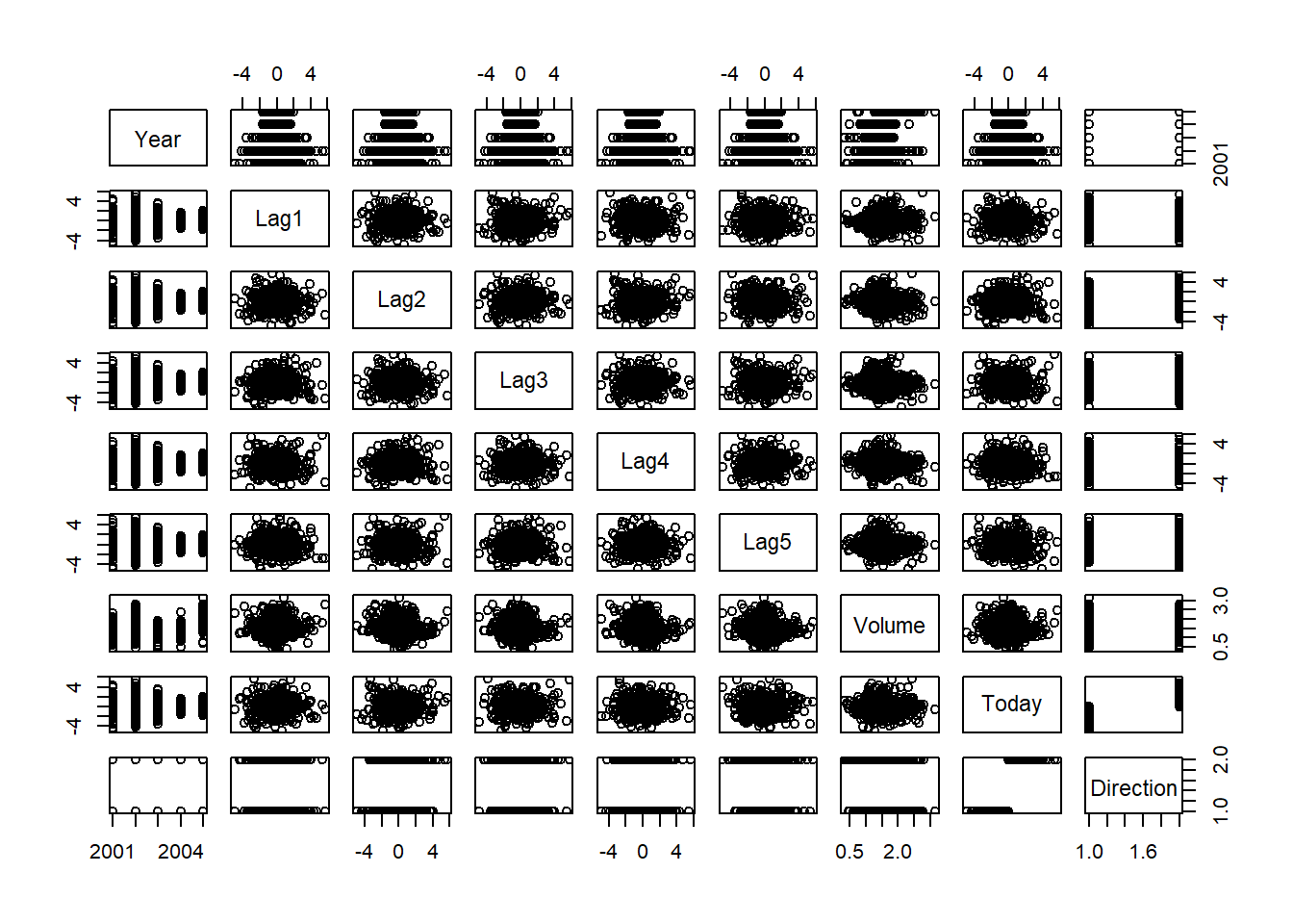
The cor() function produces a matrix that contains all
of the pairwise correlations among the predictors in a data set. The
first command below gives an error message because the
direction variable is qualitative.
cor(Smarket)## Error in cor(Smarket): 'x' must be numericcor(Smarket[, -9])## Year Lag1 Lag2 Lag3 Lag4
## Year 1.00000000 0.029699649 0.030596422 0.033194581 0.035688718
## Lag1 0.02969965 1.000000000 -0.026294328 -0.010803402 -0.002985911
## Lag2 0.03059642 -0.026294328 1.000000000 -0.025896670 -0.010853533
## Lag3 0.03319458 -0.010803402 -0.025896670 1.000000000 -0.024051036
## Lag4 0.03568872 -0.002985911 -0.010853533 -0.024051036 1.000000000
## Lag5 0.02978799 -0.005674606 -0.003557949 -0.018808338 -0.027083641
## Volume 0.53900647 0.040909908 -0.043383215 -0.041823686 -0.048414246
## Today 0.03009523 -0.026155045 -0.010250033 -0.002447647 -0.006899527
## Lag5 Volume Today
## Year 0.029787995 0.53900647 0.030095229
## Lag1 -0.005674606 0.04090991 -0.026155045
## Lag2 -0.003557949 -0.04338321 -0.010250033
## Lag3 -0.018808338 -0.04182369 -0.002447647
## Lag4 -0.027083641 -0.04841425 -0.006899527
## Lag5 1.000000000 -0.02200231 -0.034860083
## Volume -0.022002315 1.00000000 0.014591823
## Today -0.034860083 0.01459182 1.000000000As one would expect, the correlations between the lag variables and
today’s returns are close to zero. In other words, there appears to be
little correlation between today’s returns and previous days’ returns.
The only substantial correlation is between Year and
volume. By plotting the data, which is ordered
chronologically, we see that volume is increasing over
time. In other words, the average number of shares traded daily
increased from 2001 to 2005.
attach(Smarket)
plot(Volume)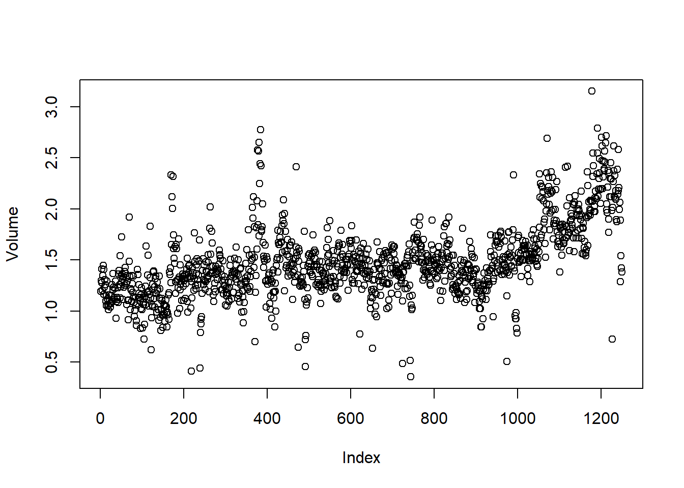
We will now perform KNN using the knn() function, which
is part of the class library. knn() forms
predictions using a single command. The function requires four
inputs.
- A matrix containing the predictors associated with the training
data, labeled
train.Xbelow. - A matrix containing the predictors associated with the data for
which we wish to make predictions, labeled
test.Xbelow. - A vector containing the class labels for the training observations,
labeled
train.Directionbelow. - A value for \(K\), the number of nearest neighbors to be used by the classifier.
We use the cbind() function, short for column
bind, to bind the Lag1 and Lag2 variables
together into two matrices, one for the training set and the other for
the test set.
library(class)
train <- (Year < 2005)
data <- cbind(Lag1, Lag2)
train.X <- data[train,]
test.X <- data[!train,]
train.Direction <- Direction[train]
test.Direction <- Direction[!train]
Now the knn() function can be used to predict the
market’s movement for the dates in 2005. We set a random seed before we
apply knn() because if several observations are tied as
nearest neighbors, then R will randomly break the tie.
Therefore, a seed must be set in order to ensure reproducibility of
results.
set.seed(1)
knn.pred <- knn(train.X, test.X, train.Direction, k = 1)
table(knn.pred, test.Direction)
## test.Direction
## knn.pred Down Up
## Down 43 58
## Up 68 83mean(knn.pred == test.Direction)## [1] 0.5The results using \(K=1\) are not very good, since only \(50\) % of the observations are correctly predicted. Of course, it may be that \(K=1\) results in an overly flexible fit to the data. Below, we repeat the analysis using \(K=3\).
set.seed(1)
knn.pred <- knn(train = train.X, test = test.X, cl = train.Direction, k = 3)
table(knn.pred, test.Direction)
## test.Direction
## knn.pred Down Up
## Down 48 55
## Up 63 86mean(knn.pred == test.Direction)## [1] 0.531746# Compare the performance of K=1 and K=3.The results have improved slightly. But increasing \(K\) further turns out to provide no further improvements.
KNN does not perform well on the Smarket data but it
does often provide impressive results. As an example we will apply the
KNN approach to the Insurance data set, which is part of
the ISLR2 library. This data set includes \(85\) predictors that measure demographic
characteristics for 5,822 individuals. The response variable is
Purchase, which indicates whether or not a given individual
purchases a caravan insurance policy. In this data set, only \(6\) % of people purchased caravan
insurance.
dim(Caravan)## [1] 5822 86attach(Caravan)
summary(Purchase)## No Yes
## 5474 348348 / 5822## [1] 0.05977327Because the KNN classifier predicts the class of a given test
observation by identifying the observations that are nearest to it, the
scale of the variables matters. Variables that are on a large scale will
have a much larger effect on the distance between the
observations, and hence on the KNN classifier, than variables that are
on a small scale. For instance, imagine a data set that contains two
variables, salary and age (measured in dollars
and years, respectively). As far as KNN is concerned, a difference of
\(\$1,000\) in salary is enormous
compared to a difference of \(50\)
years in age. Consequently, salary will drive the KNN
classification results, and age will have almost no effect.
This is contrary to our intuition that a salary difference of \(\$1,000\) is quite small compared to an age
difference of \(50\) years.
Furthermore, the importance of scale to the KNN classifier leads to
another issue: if we measured salary in Japanese yen, or if
we measured age in minutes, then we’d get quite different
classification results from what we get if these two variables are
measured in dollars and years.
A good way to handle this problem is to standardize the data
so that all variables are given a mean of zero and a standard deviation
of one. Then all variables will be on a comparable scale. The
scale() function does just this. In standardizing the data,
we exclude column \(86\), because that
is the qualitative Purchase variable.
Note that we cannot standardize the whole dataset and then split it into training and test data, because it leads to test data leakage to training data. We now first split the observations into a test set, containing the first 1,000 observations, and a training set, containing the remaining observations. Then we standardize the data with training data features’ means and standard deviations. We fit a KNN model on the training data using \(K=1\), and evaluate its performance on the test data.
test <- 1:1000
train.X <- Caravan[-test, -86]
test.X <- Caravan[test,-86]
train.X <- scale(train.X)
train_means <- attr(train.X,"scaled:center")
train_sds <- attr(train.X, "scaled:scale")
test.X <- scale(test.X, train_means, train_sds)
train.Y <- Purchase[-test]
test.Y <- Purchase[test]

set.seed(1)
knn.pred <- knn(train.X, test.X, train.Y, k = 1)
mean(test.Y != knn.pred)
## [1] 0.117mean(test.Y != "No")## [1] 0.059The vector test is numeric, with values from \(1\) through \(1,000\). Typing
Caravan[test, -86] yields the submatrix of the data
containing the observations whose indices range from \(1\) to \(1,000\), whereas typing
Caravan[-test, -86] yields the submatrix containing the
observations whose indices do not range from \(1\) to \(1,000\). The KNN error rate on the 1,000
test observations is just under \(12\)
%. At first glance, this may appear to be fairly good. However, since
only \(6\) % of customers purchased
insurance, we could get the error rate down to \(6\) % by always predicting No
regardless of the values of the predictors!
Suppose that there is some non-trivial cost to trying to sell insurance to a given individual. For instance, perhaps a salesperson must visit each potential customer. If the company tries to sell insurance to a random selection of customers, then the success rate will be only \(6\) %, which may be far too low given the costs involved. Instead, the company would like to try to sell insurance only to customers who are likely to buy it. So the overall error rate is not of interest. Instead, the fraction of individuals that are correctly predicted to buy insurance is of interest.
It turns out that KNN with \(K=1\) does far better than random guessing among the customers that are predicted to buy insurance. Among \(77\) such customers, \(9\), or \(11.7\) %, actually do purchase insurance. This is double the rate that one would obtain from random guessing.
table(knn.pred, test.Y)## test.Y
## knn.pred No Yes
## No 874 50
## Yes 67 99 / (67 + 9)## [1] 0.1184211Using \(K=3\), the success rate increases to \(23.1\) %, and with \(K=5\) the rate is also \(23.1\) %. This is over four times the rate that results from random guessing. It appears that KNN is finding some real patterns in a difficult data set!
knn.pred <- knn(train.X, test.X, train.Y, k = 3)
table(knn.pred, test.Y)
## test.Y
## knn.pred No Yes
## No 921 53
## Yes 20 66 / 26## [1] 0.2307692knn.pred <- knn(train.X, test.X, train.Y, k = 5)
table(knn.pred, test.Y)## test.Y
## knn.pred No Yes
## No 931 56
## Yes 10 33 / 13## [1] 0.2307692However, while this strategy is cost-effective, it is worth noting that only 13 customers are predicted to purchase insurance using KNN with \(K=5\). In practice, the insurance company may wish to expend resources on convincing more than just 13 potential customers to buy insurance.
Resampling Methods
In practice, we often need to evaluate model performance and choose
the best model among candidates. Resampling methods provide tools for
estimating the test error, which helps us avoid overfitting and improves
generalization. We illustrate these methods using the
Smarket dataset with KNN classification, and later with
bootstrap and (over/under)sampling examples.
train <- (Year < 2005)
data <- cbind(Lag1, Lag2)
train.X <- data[train,]
test.X <- data[!train,]
train.Direction <- Direction[train]
test.Direction <- Direction[!train]
Validation-set Approach
The validation-set approach involves splitting the available data into two parts: a training set and a validation (test) set. The model is trained on the training set and evaluated on the validation set.
In the following code, we randomly select 70% of the data for training and use the remaining 30% for testing. We then compute test error rates for different values of k in KNN.
set.seed(1)
ntrain=nrow(train.X)
pdtrainind <- sample(ntrain, 0.7*ntrain)
pdtrain.X <- train.X[pdtrainind,]
pdtest.X <- train.X[-pdtrainind,]
pdtrain.Direction <- train.Direction[pdtrainind]
pdtest.Direction <- train.Direction[-pdtrainind]
ErrTe=0; Kmax=50
for(k in 1:Kmax){
  knn.pred <- knn(train = pdtrain.X, test = pdtest.X, cl = pdtrain.Direction, k = k)
  ErrTe[k]=mean(knn.pred != pdtest.Direction)
}
plot(ErrTe,type="l")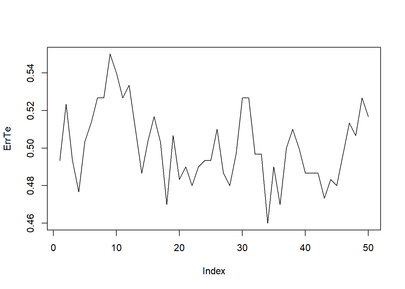
which.min(ErrTe)## [1] 34The plot shows how the error rate changes with k. The which.min(ErrTe) function returns the value of k with the lowest validation error. Repeating the split with a different random seed may give a different “optimal” k, showing that the validation-set approach can be unstable.
set.seed(2)
ntrain=nrow(train.X)
pdtrainind <- sample(ntrain, 0.7*ntrain)
pdtrain.X <- train.X[pdtrainind,]
pdtest.X <- train.X[-pdtrainind,]
pdtrain.Direction <- train.Direction[pdtrainind]
pdtest.Direction <- train.Direction[-pdtrainind]
ErrTe=0; Kmax=50
for(k in 1:Kmax){
  knn.pred <- knn(train = pdtrain.X, test = pdtest.X, cl = pdtrain.Direction, k = k)
  ErrTe[k]=mean(knn.pred != pdtest.Direction)
}
plot(ErrTe,type="l")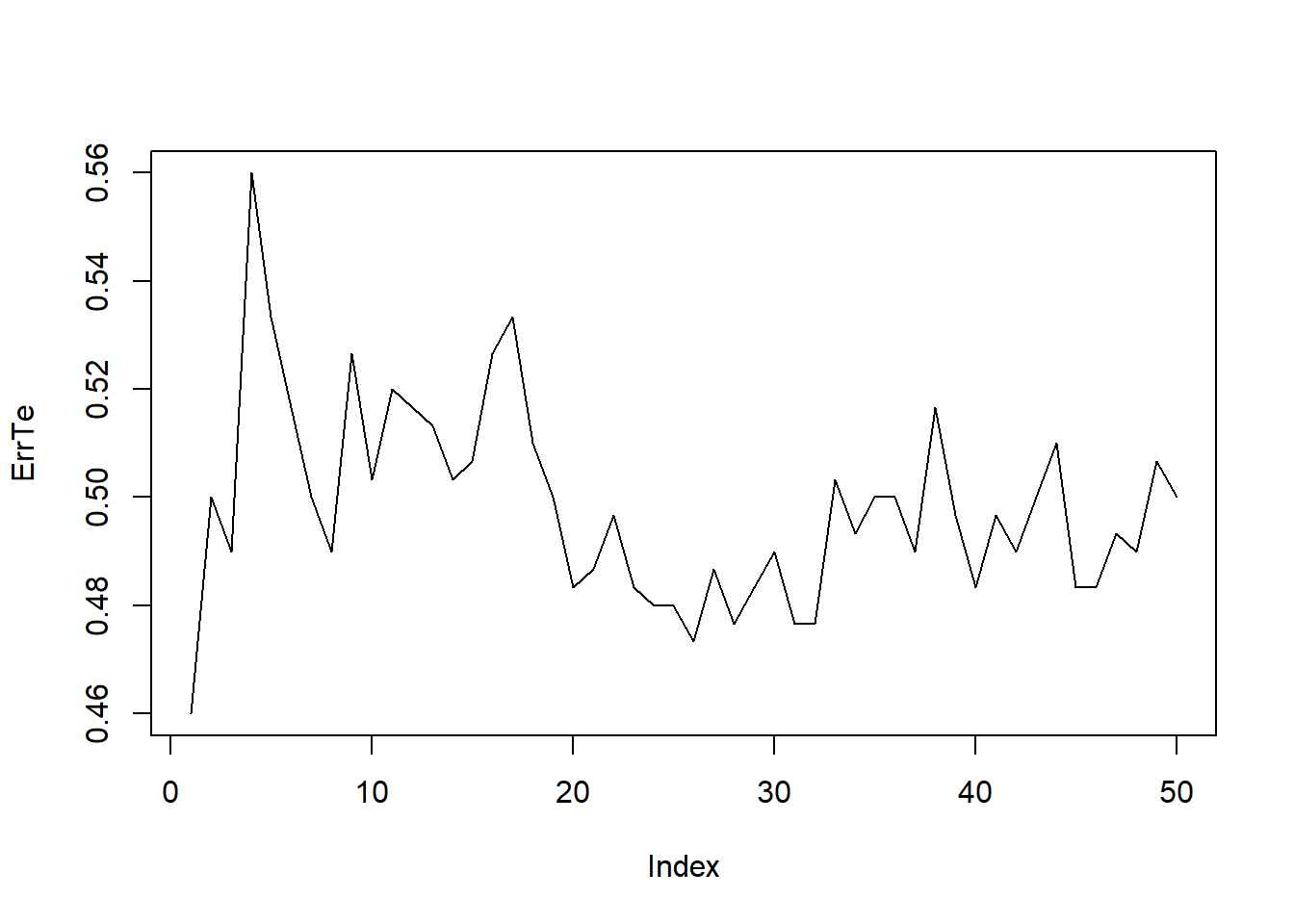
which.min(ErrTe)## [1] 1F-fold cross Validation
To obtain a more reliable estimate, we can use k-fold cross validation. The data is split into F roughly equal parts (“folds”). Each fold is used once as a validation set, while the other folds form the training set. The test errors are averaged across folds.
Here, we use 10-fold cross validation:
F <- 10
set.seed(1)
folds <- cut(seq(1,ntrain), breaks = F, labels = FALSE)
folds <- folds[sample(ntrain)]
folds
## [1] 9 7 2 10 6 5 3 3 10 2 4 6 3 9 10 5 4 8 9 6 8 1 2 8 9
## [26] 5 7 9 10 4 7 10 9 9 10 4 10 6 5 2 5 10 6 6 6 9 4 6 2 1
## [51] 7 6 4 3 2 4 1 5 9 4 3 7 6 7 1 5 1 8 8 2 4 5 2 10 8
## [76] 5 9 7 7 9 5 6 9 10 2 4 8 2 1 9 1 2 3 8 7 4 6 6 7 3
## [101] 7 2 4 5 9 9 7 5 9 9 7 6 5 8 2 4 1 10 3 7 10 9 3 2 5
## [126] 3 7 1 6 8 6 3 6 7 3 10 8 4 4 7 1 1 10 6 10 8 7 3 3 6
## [151] 4 5 1 5 4 7 4 9 9 1 4 9 3 5 8 9 9 3 8 3 2 10 10 4 5
## [176] 9 6 5 4 2 10 1 9 4 10 2 1 3 7 2 1 3 5 6 5 7 5 8 6 1
## [201] 10 8 7 7 7 2 8 6 8 10 3 5 5 2 2 10 6 10 9 3 10 6 6 9 6
## [226] 5 4 8 2 7 1 6 4 5 9 10 4 8 5 2 8 5 9 6 4 4 1 9 5 2
## [251] 9 8 5 8 9 7 3 5 10 1 6 6 1 8 3 1 10 7 1 4 9 9 7 9 7
## [276] 1 6 1 9 2 8 6 3 4 8 3 1 8 3 10 9 3 1 8 5 8 9 3 2 8
## [301] 10 3 4 7 6 9 6 5 3 4 4 8 9 6 2 7 10 9 8 7 5 2 3 5 10
## [326] 3 6 8 2 1 7 5 4 2 10 2 5 5 5 2 9 10 3 7 9 7 9 9 7 1
## [351] 1 1 5 9 10 8 5 10 1 2 2 4 5 10 3 1 5 5 2 6 2 7 5 6 9
## [376] 3 7 10 7 8 2 8 2 6 9 8 6 10 8 1 2 6 5 9 2 10 8 7 10 7
## [401] 1 6 10 7 7 1 7 4 9 5 10 6 7 6 8 6 8 10 10 8 4 3 1 10 10
## [426] 1 2 7 1 7 1 5 7 3 10 2 1 8 10 8 4 3 2 4 5 2 6 4 2 5
## [451] 5 8 4 10 9 2 9 5 2 6 4 8 10 2 1 3 3 2 8 7 4 2 8 3 2
## [476] 6 4 1 5 1 6 2 8 6 10 10 4 2 5 1 3 4 4 3 6 4 3 10 3 9
## [501] 1 8 8 7 4 7 3 6 4 1 7 1 4 10 6 9 4 10 7 7 3 2 1 7 3
## [526] 8 10 1 4 2 5 3 4 4 1 5 5 8 5 7 3 3 1 2 6 8 3 4 3 1
## [551] 10 9 6 3 8 3 9 5 3 10 9 6 5 9 7 3 3 8 10 4 1 2 6 1 4
## [576] 7 9 5 2 4 9 4 1 2 10 3 3 8 5 10 5 4 7 2 1 2 8 5 5 8
## [601] 9 9 10 3 5 10 8 6 3 4 5 3 2 1 4 1 2 6 10 1 7 9 8 5 4
## [626] 6 6 4 7 4 3 4 7 5 1 5 10 1 1 8 3 4 5 10 10 4 8 3 9 4
## [651] 10 10 7 8 6 1 8 9 7 8 10 3 7 9 8 9 5 5 10 1 5 10 3 1 6
## [676] 5 4 5 1 5 9 8 1 1 9 4 6 9 3 8 2 8 2 4 3 4 8 8 4 10
## [701] 6 1 6 6 8 5 7 8 3 4 2 5 10 10 1 6 8 6 6 6 3 4 3 6 1
## [726] 7 6 2 4 7 1 3 10 2 9 7 4 8 2 7 9 9 9 10 4 9 2 3 8 10
## [751] 2 3 7 5 6 7 3 10 2 3 9 7 6 4 5 2 10 2 5 6 10 9 1 9 8
## [776] 8 8 1 4 7 3 7 6 5 1 1 1 9 1 3 7 9 7 8 8 5 7 8 6 7
## [801] 9 5 5 9 4 7 4 4 8 6 9 10 9 8 2 3 10 7 1 7 3 10 8 7 2
## [826] 5 4 1 10 4 3 6 9 10 5 1 10 7 1 1 2 6 7 4 2 4 8 8 2 8
## [851] 1 2 2 5 2 2 8 6 10 5 7 1 9 3 8 2 2 1 9 4 3 5 1 6 3
## [876] 6 4 3 2 7 2 3 2 7 3 1 10 7 1 4 1 6 9 5 3 9 6 2 1 3
## [901] 4 6 6 4 3 8 4 7 10 5 8 6 3 5 2 6 10 5 6 9 3 5 1 8 3
## [926] 3 8 7 7 4 3 1 9 10 2 4 8 7 7 10 6 2 10 8 8 6 4 9 9 1
## [951] 5 10 2 1 9 8 10 7 8 6 10 7 2 2 5 4 2 1 2 6 10 10 1 9 6
## [976] 9 2 6 9 7 6 3 5 9 7 1 3 3 6 1 2 7 5 10 9 4 9 2We then compute the error rates for k=1,…,50 and average across folds:
Kmax=50
ErrCV <- matrix(0, nrow=F, ncol=Kmax)
for (f in 1:F) {

  # Pseudo train-test split
  pdtrainind <- which(folds != f)
  pdtrain.X <- train.X[pdtrainind,]
  pdtest.X <- train.X[-pdtrainind,]
  pdtrain.Direction <- train.Direction[pdtrainind]
  pdtest.Direction <- train.Direction[-pdtrainind]

  for(k in 1:Kmax){
    # Model fitting
    knn.pred <- knn(train = pdtrain.X, test = pdtest.X, cl = pdtrain.Direction, k = k)

    # Error
    ErrCV[f,k]=mean(knn.pred != pdtest.Direction)
  }
}
CV <- apply(ErrCV, 2, mean)
plot(CV,type="l")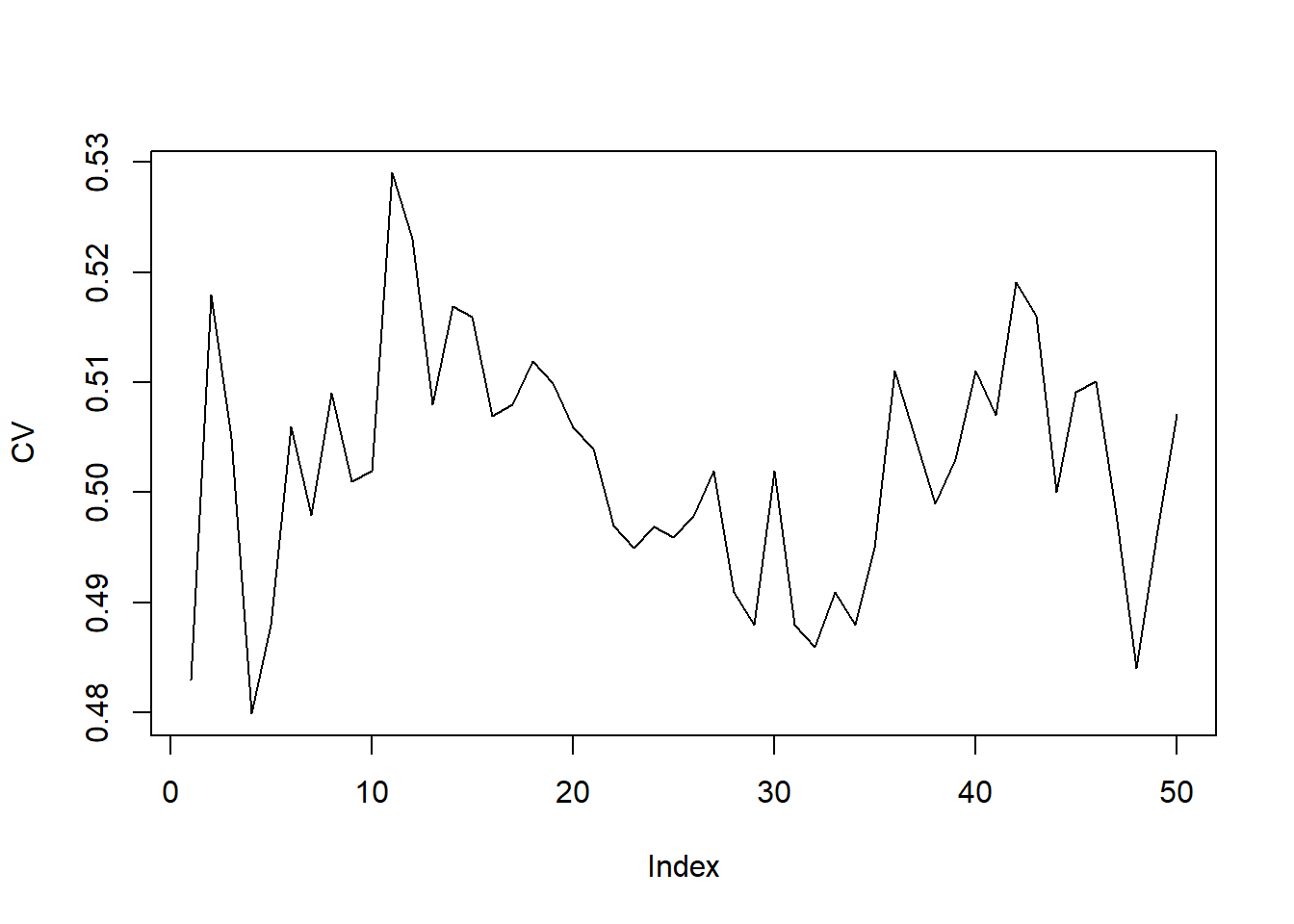
which.min(CV)## [1] 4The resulting plot typically shows a smoother curve than the
validation-set approach. The which.min(CV) gives the best
choice of k.
Bootstrap
Bootstrap is another powerful resampling technique. Instead of splitting data into folds, we generate many bootstrap datasets by sampling with replacement from the training set. Each bootstrap dataset is the same size as the original, but contains duplicate observations. This allows us to estimate variability of a statistic or model parameter.
Create one bootstrap dataset:
BSind<-sample(ntrain,replace=TRUE)
BSdata<-train.X[BSind,]
Generate multiple bootstrap datasets using a
for-loop:
B=100
for(b in 1:B){
  BSind<-sample(ntrain,replace=TRUE)
  BSdata<-train.X[BSind,]
  # ...perform analyses...
  # ...store the results indexed by b...
}
Bootstrap is particularly useful for estimating the standard error of model parameters when no analytical formula is available.
Oversampling and Undersampling
In imbalanced classification problems, where one class is much rarer than the other, resampling techniques can create a more balanced dataset.
We illustrate this with a subset of the iris dataset containing only setosa (majority) and versicolor (minority).
irisdata<-iris[1:75,]
irisdata$Species <- factor(irisdata$Species)
n<-nrow(irisdata)
majorind=(1:n)[irisdata[,5]=="setosa"]
minorind=(1:n)[irisdata[,5]=="versicolor"]
majorn=length(majorind)
minorn=length(minorind)
Oversampling duplicates minority-class samples until class sizes are equal.
OSind=sample(minorind,majorn-minorn,replace=TRUE)
OSdata<-rbind(irisdata,irisdata[OSind,])

table(irisdata$Species)
##
## setosa versicolor
## 50 25table(OSdata$Species)##
## setosa versicolor
## 50 50Undersampling removes majority-class samples to match the minority-class size.
USind=sample(majorind,majorn-minorn,replace=FALSE)
USdata<-irisdata[-USind,]

table(irisdata$Species)
##
## setosa versicolor
## 50 25table(USdata$Species)##
## setosa versicolor
## 25 25Note. Oversampling can increase the risk of overfitting (by repeating minority examples), while undersampling may discard useful information from the majority class.
SMOTE (Synthetic Minority Oversampling Technique)
In imbalanced classification problems, simply duplicating minority-class examples (oversampling) can lead to overfitting, while discarding majority-class examples (undersampling) may waste information. The SMOTE provides an alternative by generating synthetic minority observations. These new samples are created by interpolating between existing minority-class observations and their nearest neighbors.
We illustrate SMOTE using the smotefamily package on an
imbalanced version of the iris dataset, where setosa is the
majority and versicolor is the minority class.
# install.packages("smotefamily")
library(smotefamily)

# Convert to numeric labels for smotefamily
x <- irisdata[,1:4]
y <- as.numeric(irisdata$Species)  # setosa=1, versicolor=2

# Apply SMOTE
set.seed(1)
iris.SMOTE <- SMOTE(x, y, K=5, dup_size=2)

table(y)                       # original distribution
## y
## 1 2
## 50 25table(iris.SMOTE$data$class) # after SMOTE##
## 1 2
## 50 75Here: dup_size = 2 roughly doubles the minority class by
generating synthetic examples.
K = 5 specifies the number of nearest neighbors used
when interpolating new synthetic points.
The table() commands show how the class distribution
becomes more balanced after SMOTE.
Note. SMOTE creates more diverse samples than random oversampling, but if the classes overlap significantly, synthetic points may fall into ambiguous regions. Careful use of SMOTE is recommended when decision boundaries are not well-separated.