Supervised Learning II - Regression and Regularization
Patrick PUN Chi Seng (NTU Sg)
References
Chapters 3.6, 6.5.2 [ISLR2] An Introduction to Statistical Learning - with Applications in R (2nd Edition). Free access to download the book: https://www.statlearning.com/
To see the help file of a function funcname, type
?funcname.
Simple Linear Regression
The ISLR2 library’s Boston data set records
medv (median home value) for 506 census tracts along with
12 predictors such as rm (avg. rooms), age
(pre-1940 owner-occupied %), and lstat (low-SES %). We’ll
model medv using these variables.
library(MASS)
library(ISLR2)
##
## Attaching package: 'ISLR2'## The following object is masked from 'package:MASS':
##
## Bostonhead(Boston)See ?Boston for details.
We first fit a simple linear regression of medv on
lstat. The syntax is lm(y ~ x, data).
lm.fit <- lm(medv ~ lstat)## Error in eval(predvars, data, env): object 'medv' not foundThis errors because R doesn’t yet know where
medv/lstat live. Tell R to use
Boston (or attach it).
lm.fit <- lm(medv ~ lstat, data = Boston)
attach(Boston)
lm.fit <- lm(medv ~ lstat)
Print the fit for a quick glance; use summary() for coefficients, standard errors, \(R^2\), and the \(F\)-statistic.
lm.fit##
## Call:
## lm(formula = medv ~ lstat)
##
## Coefficients:
## (Intercept) lstat
## 34.55 -0.95summary(lm.fit)##
## Call:
## lm(formula = medv ~ lstat)
##
## Residuals:
## Min 1Q Median 3Q Max
## -15.168 -3.990 -1.318 2.034 24.500
##
## Coefficients:
## Estimate Std. Error t value Pr(>|t|)
## (Intercept) 34.55384 0.56263 61.41 <2e-16 ***
## lstat -0.95005 0.03873 -24.53 <2e-16 ***
## ---
## Signif. codes: 0 '***' 0.001 '**' 0.01 '*' 0.05 '.' 0.1 ' ' 1
##
## Residual standard error: 6.216 on 504 degrees of freedom
## Multiple R-squared: 0.5441, Adjusted R-squared: 0.5432
## F-statistic: 601.6 on 1 and 504 DF, p-value: < 2.2e-16Use names() to see stored components; prefer extractor
functions like coef() over $.
names(lm.fit)## [1] "coefficients" "residuals" "effects" "rank"
## [5] "fitted.values" "assign" "qr" "df.residual"
## [9] "xlevels" "call" "terms" "model"coef(lm.fit)## (Intercept) lstat
## 34.5538409 -0.9500494Confidence intervals for coefficients:
confint(lm.fit)## 2.5 % 97.5 %
## (Intercept) 33.448457 35.6592247
## lstat -1.026148 -0.8739505Predicted medv with confidence and prediction intervals
at selected lstat values:
predict(lm.fit, data.frame(lstat = (c(5, 10, 15))),
    interval = "confidence")
## fit lwr upr
## 1 29.80359 29.00741 30.59978
## 2 25.05335 24.47413 25.63256
## 3 20.30310 19.73159 20.87461predict(lm.fit, data.frame(lstat = (c(5, 10, 15))),
interval = "prediction")## fit lwr upr
## 1 29.80359 17.565675 42.04151
## 2 25.05335 12.827626 37.27907
## 3 20.30310 8.077742 32.52846For lstat = 10, the 95% confidence interval is \((24.47, 25.63)\) and the prediction
interval is \((12.828, 37.28)\): same
center, wider spread for predictions.
Plot the data and the least-squares line:
plot(lstat, medv)
abline(lm.fit)
There is visible non-linearity; we revisit this later.
abline(a, b) draws a line with intercept a
and slope b. Below are quick styling examples
(lwd, col, pch).
plot(lstat, medv)
abline(lm.fit, lwd = 3)
abline(lm.fit, lwd = 3, col = "red")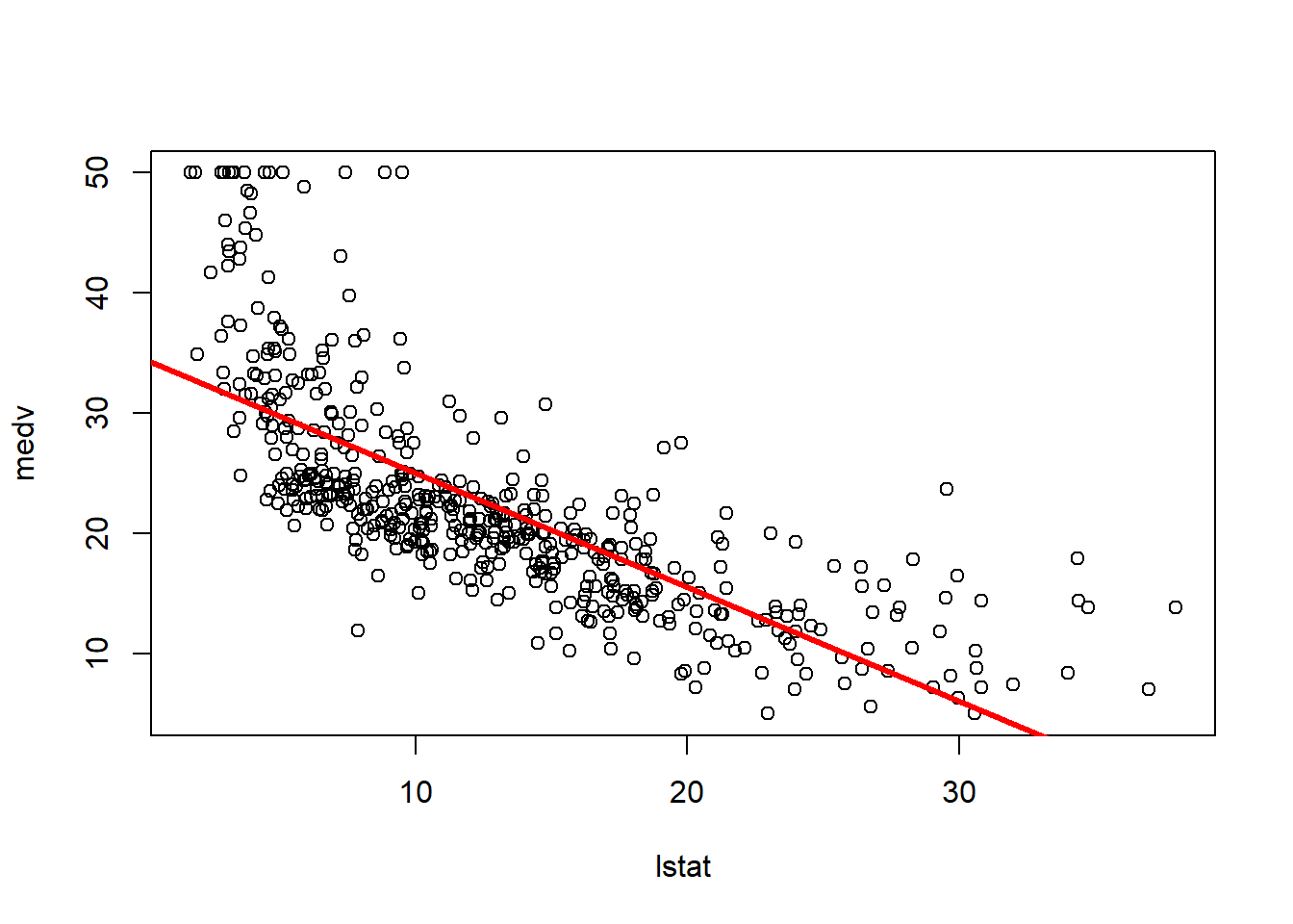
plot(lstat, medv, col = "red")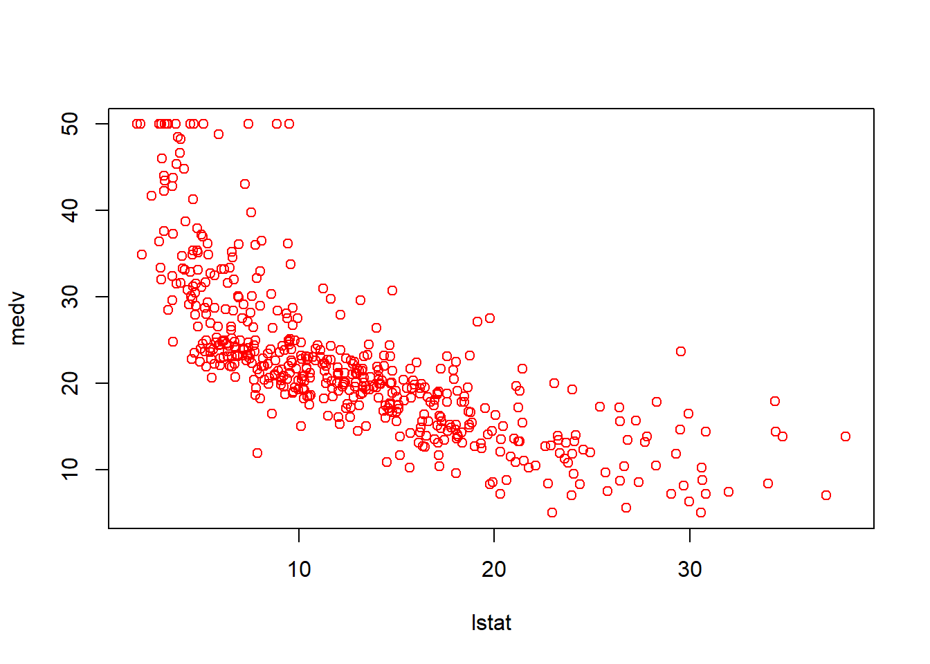
plot(lstat, medv, pch = 20)
plot(lstat, medv, pch = "+")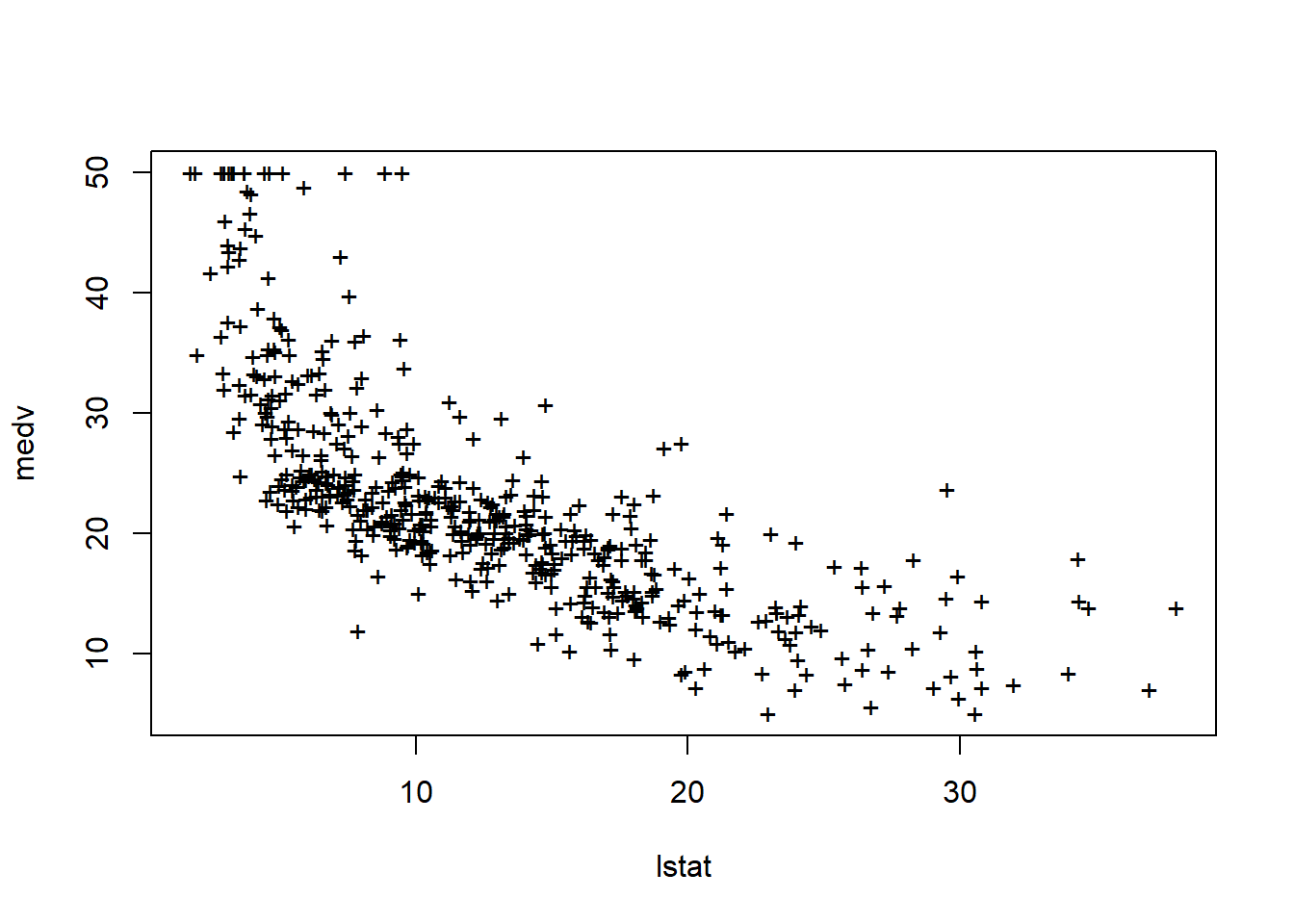
plot(1:20, 1:20, pch = 1:20)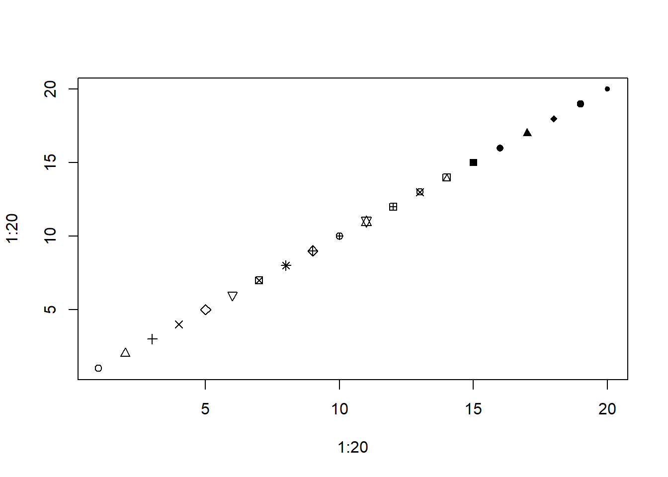
Diagnostic plots (Section 3.3.3). Use a \(2 \times 2\) grid to view all at once:
par(mfrow = c(2, 2))
plot(lm.fit)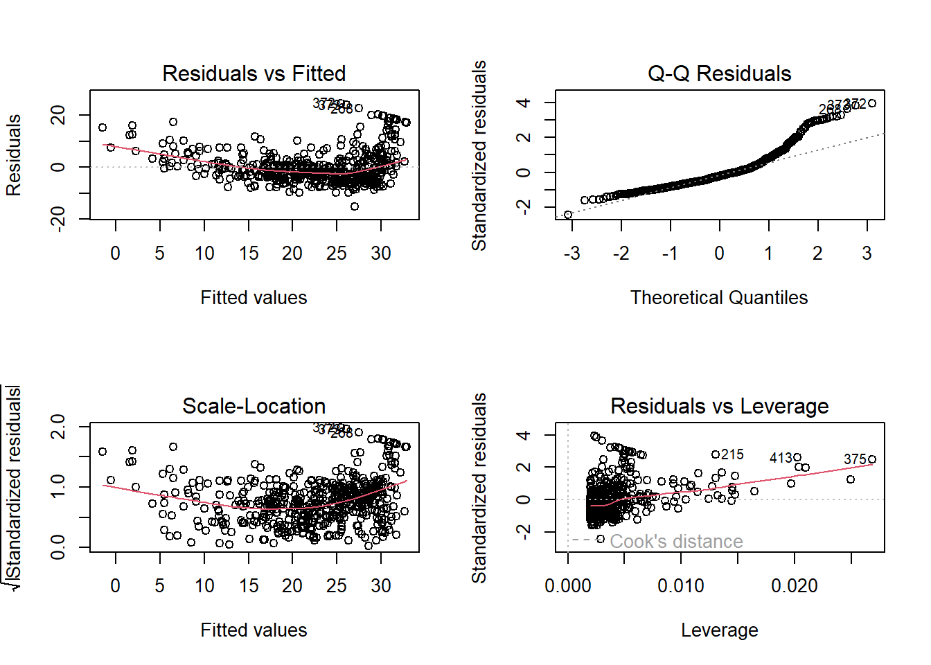
Residual diagnostics (raw and studentized) versus fitted values:
plot(predict(lm.fit), residuals(lm.fit))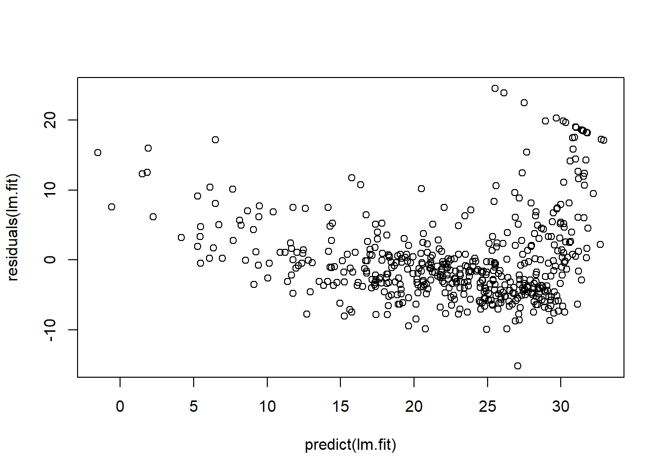
plot(predict(lm.fit), rstudent(lm.fit))
Leverage diagnostics via hat values:
plot(hatvalues(lm.fit))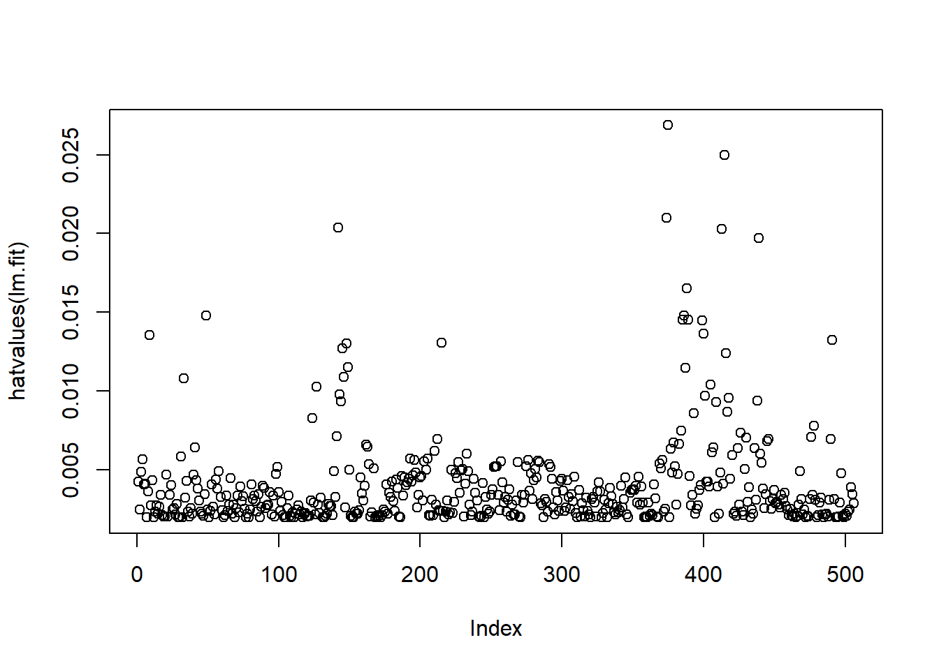
which.max(hatvalues(lm.fit))## 375
## 375which.max() returns the index of the largest
leverage.
Multiple Linear Regression
Fit multiple regression with lm(y ~ x1 + x2 + x3);
summary() reports all coefficients.
lm.fit <- lm(medv ~ lstat + age, data = Boston)
summary(lm.fit)
##
## Call:
## lm(formula = medv ~ lstat + age, data = Boston)
##
## Residuals:
## Min 1Q Median 3Q Max
## -15.981 -3.978 -1.283 1.968 23.158
##
## Coefficients:
## Estimate Std. Error t value Pr(>|t|)
## (Intercept) 33.22276 0.73085 45.458 < 2e-16 ***
## lstat -1.03207 0.04819 -21.416 < 2e-16 ***
## age 0.03454 0.01223 2.826 0.00491 **
## ---
## Signif. codes: 0 '***' 0.001 '**' 0.01 '*' 0.05 '.' 0.1 ' ' 1
##
## Residual standard error: 6.173 on 503 degrees of freedom
## Multiple R-squared: 0.5513, Adjusted R-squared: 0.5495
## F-statistic: 309 on 2 and 503 DF, p-value: < 2.2e-16Use all predictors succinctly with .:
lm.fit <- lm(medv ~ ., data = Boston)
summary(lm.fit)
##
## Call:
## lm(formula = medv ~ ., data = Boston)
##
## Residuals:
## Min 1Q Median 3Q Max
## -15.1304 -2.7673 -0.5814 1.9414 26.2526
##
## Coefficients:
## Estimate Std. Error t value Pr(>|t|)
## (Intercept) 41.617270 4.936039 8.431 3.79e-16 ***
## crim -0.121389 0.033000 -3.678 0.000261 ***
## zn 0.046963 0.013879 3.384 0.000772 ***
## indus 0.013468 0.062145 0.217 0.828520
## chas 2.839993 0.870007 3.264 0.001173 **
## nox -18.758022 3.851355 -4.870 1.50e-06 ***
## rm 3.658119 0.420246 8.705 < 2e-16 ***
## age 0.003611 0.013329 0.271 0.786595
## dis -1.490754 0.201623 -7.394 6.17e-13 ***
## rad 0.289405 0.066908 4.325 1.84e-05 ***
## tax -0.012682 0.003801 -3.337 0.000912 ***
## ptratio -0.937533 0.132206 -7.091 4.63e-12 ***
## lstat -0.552019 0.050659 -10.897 < 2e-16 ***
## ---
## Signif. codes: 0 '***' 0.001 '**' 0.01 '*' 0.05 '.' 0.1 ' ' 1
##
## Residual standard error: 4.798 on 493 degrees of freedom
## Multiple R-squared: 0.7343, Adjusted R-squared: 0.7278
## F-statistic: 113.5 on 12 and 493 DF, p-value: < 2.2e-16Exclude a predictor (e.g., age) using formula shorthand
or update():
lm.fit1 <- lm(medv ~ . - age, data = Boston)
summary(lm.fit1)
##
## Call:
## lm(formula = medv ~ . - age, data = Boston)
##
## Residuals:
## Min 1Q Median 3Q Max
## -15.1851 -2.7330 -0.6116 1.8555 26.3838
##
## Coefficients:
## Estimate Std. Error t value Pr(>|t|)
## (Intercept) 41.525128 4.919684 8.441 3.52e-16 ***
## crim -0.121426 0.032969 -3.683 0.000256 ***
## zn 0.046512 0.013766 3.379 0.000785 ***
## indus 0.013451 0.062086 0.217 0.828577
## chas 2.852773 0.867912 3.287 0.001085 **
## nox -18.485070 3.713714 -4.978 8.91e-07 ***
## rm 3.681070 0.411230 8.951 < 2e-16 ***
## dis -1.506777 0.192570 -7.825 3.12e-14 ***
## rad 0.287940 0.066627 4.322 1.87e-05 ***
## tax -0.012653 0.003796 -3.333 0.000923 ***
## ptratio -0.934649 0.131653 -7.099 4.39e-12 ***
## lstat -0.547409 0.047669 -11.483 < 2e-16 ***
## ---
## Signif. codes: 0 '***' 0.001 '**' 0.01 '*' 0.05 '.' 0.1 ' ' 1
##
## Residual standard error: 4.794 on 494 degrees of freedom
## Multiple R-squared: 0.7343, Adjusted R-squared: 0.7284
## F-statistic: 124.1 on 11 and 494 DF, p-value: < 2.2e-16lm.fit1 <- update(lm.fit, ~ . - age)Interaction Terms
Include interactions with : or * (the
latter expands to main effects + interaction):
summary(lm(medv ~ lstat * age, data = Boston))##
## Call:
## lm(formula = medv ~ lstat * age, data = Boston)
##
## Residuals:
## Min 1Q Median 3Q Max
## -15.806 -4.045 -1.333 2.085 27.552
##
## Coefficients:
## Estimate Std. Error t value Pr(>|t|)
## (Intercept) 36.0885359 1.4698355 24.553 < 2e-16 ***
## lstat -1.3921168 0.1674555 -8.313 8.78e-16 ***
## age -0.0007209 0.0198792 -0.036 0.9711
## lstat:age 0.0041560 0.0018518 2.244 0.0252 *
## ---
## Signif. codes: 0 '***' 0.001 '**' 0.01 '*' 0.05 '.' 0.1 ' ' 1
##
## Residual standard error: 6.149 on 502 degrees of freedom
## Multiple R-squared: 0.5557, Adjusted R-squared: 0.5531
## F-statistic: 209.3 on 3 and 502 DF, p-value: < 2.2e-16Non-linear Transformations of the Predictors
Create polynomial terms with I(X^2) (the
I() ensures exponentiation inside formulas). Fit a
quadratic in lstat:
lm.fit2 <- lm(medv ~ lstat + I(lstat^2))
summary(lm.fit2)
##
## Call:
## lm(formula = medv ~ lstat + I(lstat^2))
##
## Residuals:
## Min 1Q Median 3Q Max
## -15.2834 -3.8313 -0.5295 2.3095 25.4148
##
## Coefficients:
## Estimate Std. Error t value Pr(>|t|)
## (Intercept) 42.862007 0.872084 49.15 <2e-16 ***
## lstat -2.332821 0.123803 -18.84 <2e-16 ***
## I(lstat^2) 0.043547 0.003745 11.63 <2e-16 ***
## ---
## Signif. codes: 0 '***' 0.001 '**' 0.01 '*' 0.05 '.' 0.1 ' ' 1
##
## Residual standard error: 5.524 on 503 degrees of freedom
## Multiple R-squared: 0.6407, Adjusted R-squared: 0.6393
## F-statistic: 448.5 on 2 and 503 DF, p-value: < 2.2e-16Quadratic terms markedly improve fit; residuals look cleaner:
par(mfrow = c(2, 2))
plot(lm.fit2)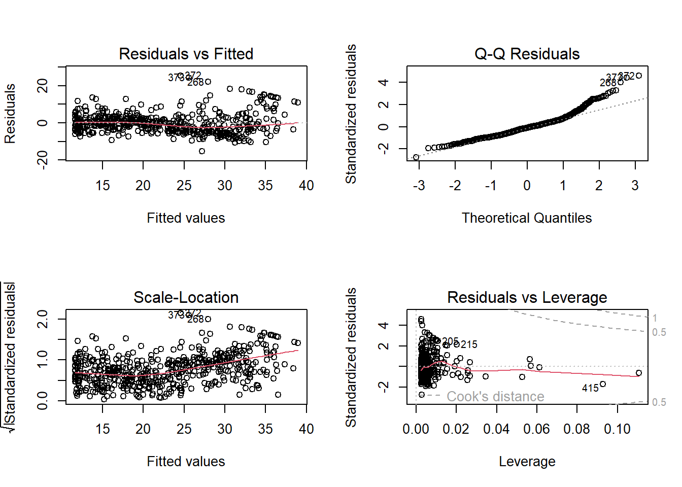
Higher-order polynomials via poly() (orthogonal by
default). Fifth-order example:
lm.fit5 <- lm(medv ~ poly(lstat, 5))
summary(lm.fit5)
##
## Call:
## lm(formula = medv ~ poly(lstat, 5))
##
## Residuals:
## Min 1Q Median 3Q Max
## -13.5433 -3.1039 -0.7052 2.0844 27.1153
##
## Coefficients:
## Estimate Std. Error t value Pr(>|t|)
## (Intercept) 22.5328 0.2318 97.197 < 2e-16 ***
## poly(lstat, 5)1 -152.4595 5.2148 -29.236 < 2e-16 ***
## poly(lstat, 5)2 64.2272 5.2148 12.316 < 2e-16 ***
## poly(lstat, 5)3 -27.0511 5.2148 -5.187 3.10e-07 ***
## poly(lstat, 5)4 25.4517 5.2148 4.881 1.42e-06 ***
## poly(lstat, 5)5 -19.2524 5.2148 -3.692 0.000247 ***
## ---
## Signif. codes: 0 '***' 0.001 '**' 0.01 '*' 0.05 '.' 0.1 ' ' 1
##
## Residual standard error: 5.215 on 500 degrees of freedom
## Multiple R-squared: 0.6817, Adjusted R-squared: 0.6785
## F-statistic: 214.2 on 5 and 500 DF, p-value: < 2.2e-16Orthogonal polynomials change coefficient interpretation but not
fitted values versus raw powers; use raw = TRUE for raw
polynomials.
Log transforms are also possible:
summary(lm(medv ~ log(rm), data = Boston))##
## Call:
## lm(formula = medv ~ log(rm), data = Boston)
##
## Residuals:
## Min 1Q Median 3Q Max
## -19.487 -2.875 -0.104 2.837 39.816
##
## Coefficients:
## Estimate Std. Error t value Pr(>|t|)
## (Intercept) -76.488 5.028 -15.21 <2e-16 ***
## log(rm) 54.055 2.739 19.73 <2e-16 ***
## ---
## Signif. codes: 0 '***' 0.001 '**' 0.01 '*' 0.05 '.' 0.1 ' ' 1
##
## Residual standard error: 6.915 on 504 degrees of freedom
## Multiple R-squared: 0.4358, Adjusted R-squared: 0.4347
## F-statistic: 389.3 on 1 and 504 DF, p-value: < 2.2e-16Qualitative Predictors
The Carseats data include qualitative predictors like
ShelveLoc (Bad/Medium/Good). R creates dummy variables
automatically; we can include interactions too.
head(Carseats)lm.fit <- lm(Sales ~ . + Income:Advertising + Price:Age, data = Carseats)
summary(lm.fit)##
## Call:
## lm(formula = Sales ~ . + Income:Advertising + Price:Age, data = Carseats)
##
## Residuals:
## Min 1Q Median 3Q Max
## -2.9208 -0.7503 0.0177 0.6754 3.3413
##
## Coefficients:
## Estimate Std. Error t value Pr(>|t|)
## (Intercept) 6.5755654 1.0087470 6.519 2.22e-10 ***
## CompPrice 0.0929371 0.0041183 22.567 < 2e-16 ***
## Income 0.0108940 0.0026044 4.183 3.57e-05 ***
## Advertising 0.0702462 0.0226091 3.107 0.002030 **
## Population 0.0001592 0.0003679 0.433 0.665330
## Price -0.1008064 0.0074399 -13.549 < 2e-16 ***
## ShelveLocGood 4.8486762 0.1528378 31.724 < 2e-16 ***
## ShelveLocMedium 1.9532620 0.1257682 15.531 < 2e-16 ***
## Age -0.0579466 0.0159506 -3.633 0.000318 ***
## Education -0.0208525 0.0196131 -1.063 0.288361
## UrbanYes 0.1401597 0.1124019 1.247 0.213171
## USYes -0.1575571 0.1489234 -1.058 0.290729
## Income:Advertising 0.0007510 0.0002784 2.698 0.007290 **
## Price:Age 0.0001068 0.0001333 0.801 0.423812
## ---
## Signif. codes: 0 '***' 0.001 '**' 0.01 '*' 0.05 '.' 0.1 ' ' 1
##
## Residual standard error: 1.011 on 386 degrees of freedom
## Multiple R-squared: 0.8761, Adjusted R-squared: 0.8719
## F-statistic: 210 on 13 and 386 DF, p-value: < 2.2e-16Inspect dummy coding with contrasts():
attach(Carseats)
contrasts(ShelveLoc)
## Good Medium
## Bad 0 0
## Good 1 0
## Medium 0 1By default, Bad is the baseline; positive coefficients for
ShelveLocGood and ShelveLocMedium indicate
higher sales relative to Bad (with Good > Medium). See
?contrasts for alternative codings.
Regularization: Ridge Regression and the Lasso
Here we apply regularization to the Hitters data, aiming
to predict a baseball player’s Salary from performance
statistics in the previous year.
The Salary variable contains missing values. The
is.na() function flags missing entries with
TRUE, and sum() counts them.
library(ISLR2)
names(Hitters)
## [1] "AtBat" "Hits" "HmRun" "Runs" "RBI" "Walks"
## [7] "Years" "CAtBat" "CHits" "CHmRun" "CRuns" "CRBI"
## [13] "CWalks" "League" "Division" "PutOuts" "Assists" "Errors"
## [19] "Salary" "NewLeague"dim(Hitters)## [1] 322 20sum(is.na(Hitters$Salary))## [1] 59We find that Salary is missing for 59 players. To
proceed, we remove rows with missing values using
na.omit().
Hitters <- na.omit(Hitters)
dim(Hitters)
## [1] 263 20sum(is.na(Hitters))## [1] 0We will use the glmnet package in order to perform ridge
regression and the lasso. The main function in this package is
glmnet(), which can be used to fit ridge regression models,
lasso models, and more.
We use the glmnet package for ridge regression and the
lasso. The main function glmnet() fits both models but uses
different syntax: we must pass an x matrix of predictors
and a y response vector, rather than a formula. Before
proceeding, ensure missing values are removed from Hitters
(see Section 6.5.1).
x <- model.matrix(Salary ~ ., Hitters)[, -1]
y <- Hitters$Salary
model.matrix() conveniently creates x: it
includes the 19 predictors and automatically converts qualitative
variables into dummies. This is essential since glmnet()
only accepts numeric inputs.
Ridge Regression
library(glmnet)## Loading required package: Matrix## Loaded glmnet 4.1-10grid <- 10^seq(10, -2, length = 100)
ridge.mod <- glmnet(x, y, alpha = 0, lambda = grid, standardize = TRUE)By default, glmnet() selects its own grid of \(\lambda\) values; here we specify one
ranging from \(10^{10}\) to \(10^{-2}\). This spans from the
intercept-only model to least squares. Variables are standardized by
default (standardize=FALSE disables this).
Each \(\lambda\) has an associated coefficient vector stored in a \(20 \times 100\) matrix: 20 rows (19 predictors + intercept), 100 columns (grid values).
dim(coef(ridge.mod))## [1] 20 100Coefficient norms shrink with larger \(\lambda\). For \(\lambda=11,498\):
ridge.mod$lambda[50]## [1] 11497.57coef(ridge.mod)[, 50]## (Intercept) AtBat Hits HmRun Runs
## 407.356050200 0.036957182 0.138180344 0.524629976 0.230701523
## RBI Walks Years CAtBat CHits
## 0.239841459 0.289618741 1.107702929 0.003131815 0.011653637
## CHmRun CRuns CRBI CWalks LeagueN
## 0.087545670 0.023379882 0.024138320 0.025015421 0.085028114
## DivisionW PutOuts Assists Errors NewLeagueN
## -6.215440973 0.016482577 0.002612988 -0.020502690 0.301433531sqrt(sum(coef(ridge.mod)[-1, 50]^2))## [1] 6.360612For \(\lambda=705\), the \(\ell_2\) norm is much larger:
ridge.mod$lambda[60]## [1] 705.4802coef(ridge.mod)[, 60]## (Intercept) AtBat Hits HmRun Runs RBI
## 54.32519950 0.11211115 0.65622409 1.17980910 0.93769713 0.84718546
## Walks Years CAtBat CHits CHmRun CRuns
## 1.31987948 2.59640425 0.01083413 0.04674557 0.33777318 0.09355528
## CRBI CWalks LeagueN DivisionW PutOuts Assists
## 0.09780402 0.07189612 13.68370191 -54.65877750 0.11852289 0.01606037
## Errors NewLeagueN
## -0.70358655 8.61181213sqrt(sum(coef(ridge.mod)[-1, 60]^2))## [1] 57.11001We can obtain coefficients for any \(\lambda\), even if not in the original grid:
predict(ridge.mod, s = 50, type = "coefficients")[1:20, ]## (Intercept) AtBat Hits HmRun Runs
## 4.876610e+01 -3.580999e-01 1.969359e+00 -1.278248e+00 1.145892e+00
## RBI Walks Years CAtBat CHits
## 8.038292e-01 2.716186e+00 -6.218319e+00 5.447837e-03 1.064895e-01
## CHmRun CRuns CRBI CWalks LeagueN
## 6.244860e-01 2.214985e-01 2.186914e-01 -1.500245e-01 4.592589e+01
## DivisionW PutOuts Assists Errors NewLeagueN
## -1.182011e+02 2.502322e-01 1.215665e-01 -3.278600e+00 -9.496680e+00Next we split the data into training and test sets to estimate test error. One way is to randomly select half the observations for training.
set.seed(1)
train <- sample(1:nrow(x), nrow(x)/2)
test <- (-train)
y.test <- y[test]
Fit ridge on the training set and evaluate MSE on the test set at \(\lambda=4\):
ridge.mod <- glmnet(x[train, ], y[train], alpha = 0, lambda = grid, thresh = 1e-12, standardize = TRUE)
ridge.pred <- predict(ridge.mod, s = 4, newx = x[test, ])
mean((ridge.pred - y.test)^2)
## [1] 142199.2The test MSE is 142,199. If we had fit only an intercept, the prediction would be the training mean:
mean((mean(y[train]) - y.test)^2)## [1] 224669.9This matches ridge with a very large \(\lambda\):
ridge.pred <- predict(ridge.mod, s = 1e10, newx = x[test, ])
mean((ridge.pred - y.test)^2)
## [1] 224669.8Thus \(\lambda=4\) yields a far
lower test MSE than the null model. But is it better than least squares?
Recall least squares is ridge with \(\lambda=0\). With exact=TRUE,
glmnet() reproduces the least squares fit:
ridge.pred <- predict(ridge.mod, s = 0, newx = x[test, ], exact = T, x = x[train, ], y = y[train])
mean((ridge.pred - y.test)^2)
## [1] 168588.6lm(y ~ x, subset = train)##
## Call:
## lm(formula = y ~ x, subset = train)
##
## Coefficients:
## (Intercept) xAtBat xHits xHmRun xRuns xRBI
## 274.0145 -0.3521 -1.6377 5.8145 1.5424 1.1243
## xWalks xYears xCAtBat xCHits xCHmRun xCRuns
## 3.7287 -16.3773 -0.6412 3.1632 3.4008 -0.9739
## xCRBI xCWalks xLeagueN xDivisionW xPutOuts xAssists
## -0.6005 0.3379 119.1486 -144.0831 0.1976 0.6804
## xErrors xNewLeagueN
## -4.7128 -71.0951predict(ridge.mod, s = 0, exact = T, type = "coefficients",
x = x[train, ], y = y[train])[1:20, ]## (Intercept) AtBat Hits HmRun Runs RBI
## 274.0200994 -0.3521900 -1.6371383 5.8146692 1.5423361 1.1241837
## Walks Years CAtBat CHits CHmRun CRuns
## 3.7288406 -16.3795195 -0.6411235 3.1629444 3.4005281 -0.9739405
## CRBI CWalks LeagueN DivisionW PutOuts Assists
## -0.6003976 0.3378422 119.1434637 -144.0853061 0.1976300 0.6804200
## Errors NewLeagueN
## -4.7127879 -71.0898914In practice, use lm() for unpenalized regression, since
it provides standard errors and p-values.
Rather than fixing \(\lambda=4\),
cross-validation gives a better choice. cv.glmnet()
performs (by default) 10-fold CV. Set a seed for reproducibility.
set.seed(1)
cv.out <- cv.glmnet(x[train, ], y[train], alpha = 0, standardize = TRUE)
plot(cv.out)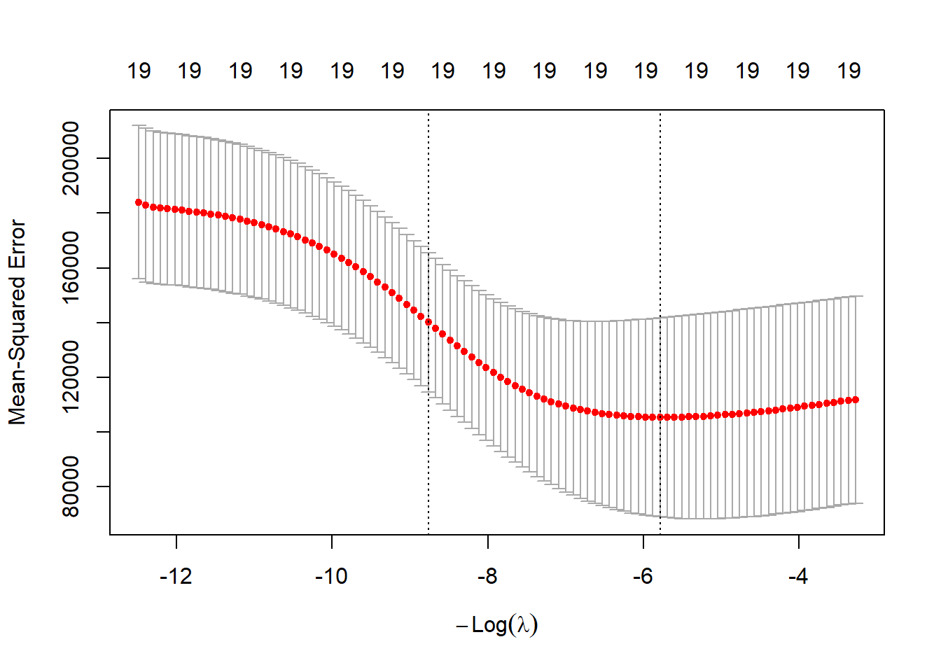
bestlam <- cv.out$lambda.min
bestlam
## [1] 326.0828The best \(\lambda\) is 326. The test MSE is:
ridge.pred <- predict(ridge.mod, s = bestlam, newx = x[test, ])
mean((ridge.pred - y.test)^2)
## [1] 139856.6This improves over \(\lambda=4\). Finally, refit ridge on the full data using the CV \(\lambda\):
out <- glmnet(x, y, alpha = 0, standardize = TRUE)
predict(out, type = "coefficients", s = bestlam)[1:20, ]
## (Intercept) AtBat Hits HmRun Runs RBI
## 15.44383120 0.07715547 0.85911582 0.60103106 1.06369007 0.87936105
## Walks Years CAtBat CHits CHmRun CRuns
## 1.62444617 1.35254778 0.01134999 0.05746654 0.40680157 0.11456224
## CRBI CWalks LeagueN DivisionW PutOuts Assists
## 0.12116504 0.05299202 22.09143197 -79.04032656 0.16619903 0.02941950
## Errors NewLeagueN
## -1.36092945 9.12487765As expected, no coefficients are exactly zero: ridge does not perform variable selection.
The Lasso
Can the lasso produce a more accurate or sparser model? Fit it with
alpha=1:
lasso.mod <- glmnet(x[train, ], y[train], alpha = 1, lambda = grid, standardize = TRUE)
plot(lasso.mod)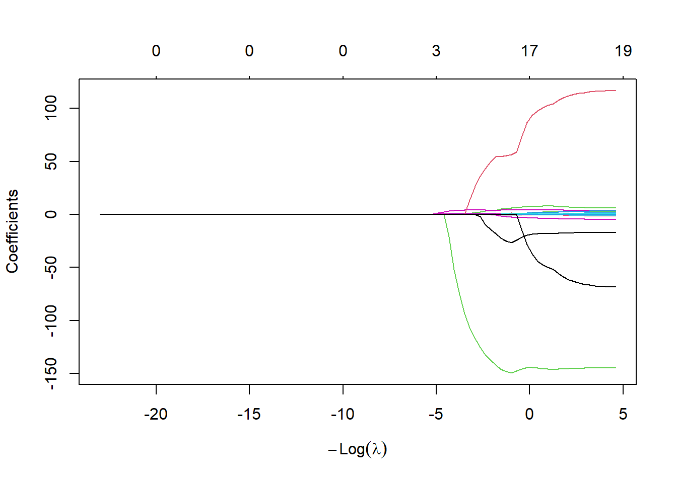
The coefficient plot shows some coefficients shrink exactly to zero, depending on \(\lambda\). Use cross-validation to choose \(\lambda\):
set.seed(1)
cv.out <- cv.glmnet(x[train, ], y[train], alpha = 1, standardize = TRUE)
plot(cv.out)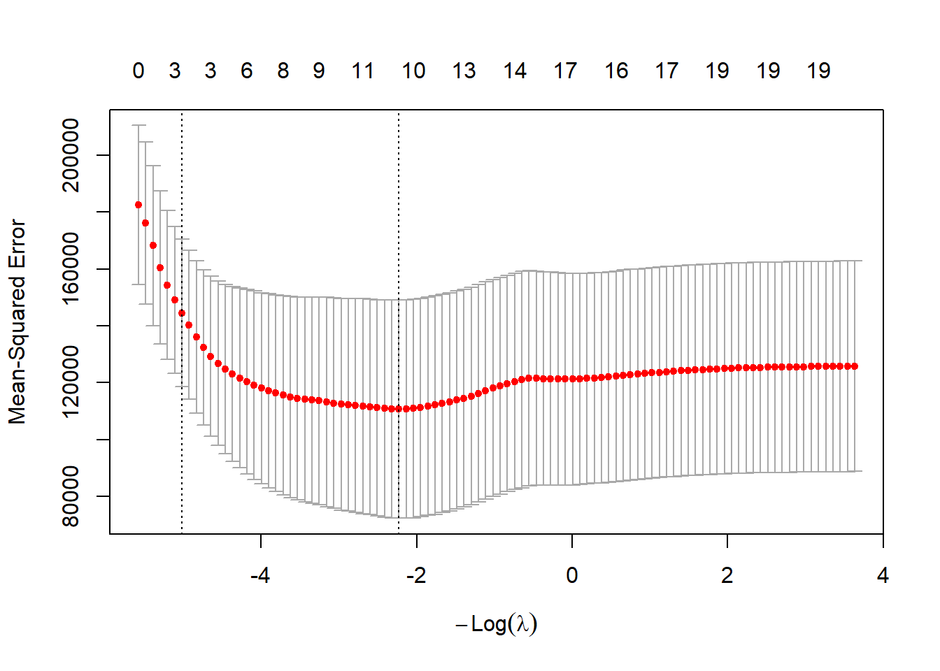
bestlam <- cv.out$lambda.min
lasso.pred <- predict(lasso.mod, s = bestlam, newx = x[test, ])
mean((lasso.pred - y.test)^2)
## [1] 143673.6The lasso test MSE is similar to ridge with CV \(\lambda\), but with the advantage of sparsity: 8 of 19 predictors are set to zero.
out <- glmnet(x, y, alpha = 1, lambda = grid, standardize = TRUE)
lasso.coef <- predict(out, type = "coefficients", s = bestlam)[1:20, ]
lasso.coef
## (Intercept) AtBat Hits HmRun Runs
## 1.27479059 -0.05497143 2.18034583 0.00000000 0.00000000
## RBI Walks Years CAtBat CHits
## 0.00000000 2.29192406 -0.33806109 0.00000000 0.00000000
## CHmRun CRuns CRBI CWalks LeagueN
## 0.02825013 0.21628385 0.41712537 0.00000000 20.28615023
## DivisionW PutOuts Assists Errors NewLeagueN
## -116.16755870 0.23752385 0.00000000 -0.85629148 0.00000000lasso.coef[lasso.coef != 0]## (Intercept) AtBat Hits Walks Years
## 1.27479059 -0.05497143 2.18034583 2.29192406 -0.33806109
## CHmRun CRuns CRBI LeagueN DivisionW
## 0.02825013 0.21628385 0.41712537 20.28615023 -116.16755870
## PutOuts Errors
## 0.23752385 -0.85629148(Self-study) Appendix: Subset Selection Methods
Best Subset Selection
The regsubsets() function (part of the
leaps library) performs best subset selection by
identifying the best model that contains a given number of predictors,
where best is quantified using RSS. The syntax is the same as
for lm(). The summary() command outputs the
best set of variables for each model size.
library(leaps)
regfit.full <- regsubsets(Salary ~ ., Hitters)
summary(regfit.full)
## Subset selection object
## Call: regsubsets.formula(Salary ~ ., Hitters)
## 19 Variables (and intercept)
## Forced in Forced out
## AtBat FALSE FALSE
## Hits FALSE FALSE
## HmRun FALSE FALSE
## Runs FALSE FALSE
## RBI FALSE FALSE
## Walks FALSE FALSE
## Years FALSE FALSE
## CAtBat FALSE FALSE
## CHits FALSE FALSE
## CHmRun FALSE FALSE
## CRuns FALSE FALSE
## CRBI FALSE FALSE
## CWalks FALSE FALSE
## LeagueN FALSE FALSE
## DivisionW FALSE FALSE
## PutOuts FALSE FALSE
## Assists FALSE FALSE
## Errors FALSE FALSE
## NewLeagueN FALSE FALSE
## 1 subsets of each size up to 8
## Selection Algorithm: exhaustive
## AtBat Hits HmRun Runs RBI Walks Years CAtBat CHits CHmRun CRuns CRBI
## 1 ( 1 ) " " " " " " " " " " " " " " " " " " " " " " "*"
## 2 ( 1 ) " " "*" " " " " " " " " " " " " " " " " " " "*"
## 3 ( 1 ) " " "*" " " " " " " " " " " " " " " " " " " "*"
## 4 ( 1 ) " " "*" " " " " " " " " " " " " " " " " " " "*"
## 5 ( 1 ) "*" "*" " " " " " " " " " " " " " " " " " " "*"
## 6 ( 1 ) "*" "*" " " " " " " "*" " " " " " " " " " " "*"
## 7 ( 1 ) " " "*" " " " " " " "*" " " "*" "*" "*" " " " "
## 8 ( 1 ) "*" "*" " " " " " " "*" " " " " " " "*" "*" " "
## CWalks LeagueN DivisionW PutOuts Assists Errors NewLeagueN
## 1 ( 1 ) " " " " " " " " " " " " " "
## 2 ( 1 ) " " " " " " " " " " " " " "
## 3 ( 1 ) " " " " " " "*" " " " " " "
## 4 ( 1 ) " " " " "*" "*" " " " " " "
## 5 ( 1 ) " " " " "*" "*" " " " " " "
## 6 ( 1 ) " " " " "*" "*" " " " " " "
## 7 ( 1 ) " " " " "*" "*" " " " " " "
## 8 ( 1 ) "*" " " "*" "*" " " " " " "An asterisk indicates that a given variable is included in the
corresponding model. For instance, this output indicates that the best
two-variable model contains only Hits and
CRBI. By default, regsubsets() only reports
results up to the best eight-variable model. But the nvmax
option can be used in order to return as many variables as are desired.
Here we fit up to a 19-variable model.
regfit.full <- regsubsets(Salary ~ ., data = Hitters, nvmax = 19)
reg.summary <- summary(regfit.full)
The summary() function also returns \(R^2\), RSS, adjusted \(R^2\), \(C_p\), and BIC. We can examine these to try
to select the best overall model.
names(reg.summary)## [1] "which" "rsq" "rss" "adjr2" "cp" "bic" "outmat" "obj"For instance, we see that the \(R^2\) statistic increases from \(32 \%\), when only one variable is included in the model, to almost \(55 \%\), when all variables are included. As expected, the \(R^2\) statistic increases monotonically as more variables are included.
reg.summary$rsq## [1] 0.3214501 0.4252237 0.4514294 0.4754067 0.4908036 0.5087146 0.5141227
## [8] 0.5285569 0.5346124 0.5404950 0.5426153 0.5436302 0.5444570 0.5452164
## [15] 0.5454692 0.5457656 0.5459518 0.5460945 0.5461159Plotting RSS, adjusted \(R^2\),
\(C_p\), and BIC for all of the models
at once will help us decide which model to select. Note the
type = "l" option tells R to connect the
plotted points with lines.
par(mfrow = c(1, 2))
plot(reg.summary$rss, xlab = "Number of Variables", ylab = "RSS", type = "l")
plot(reg.summary$adjr2, xlab = "Number of Variables", ylab = "Adjusted RSq", type = "l")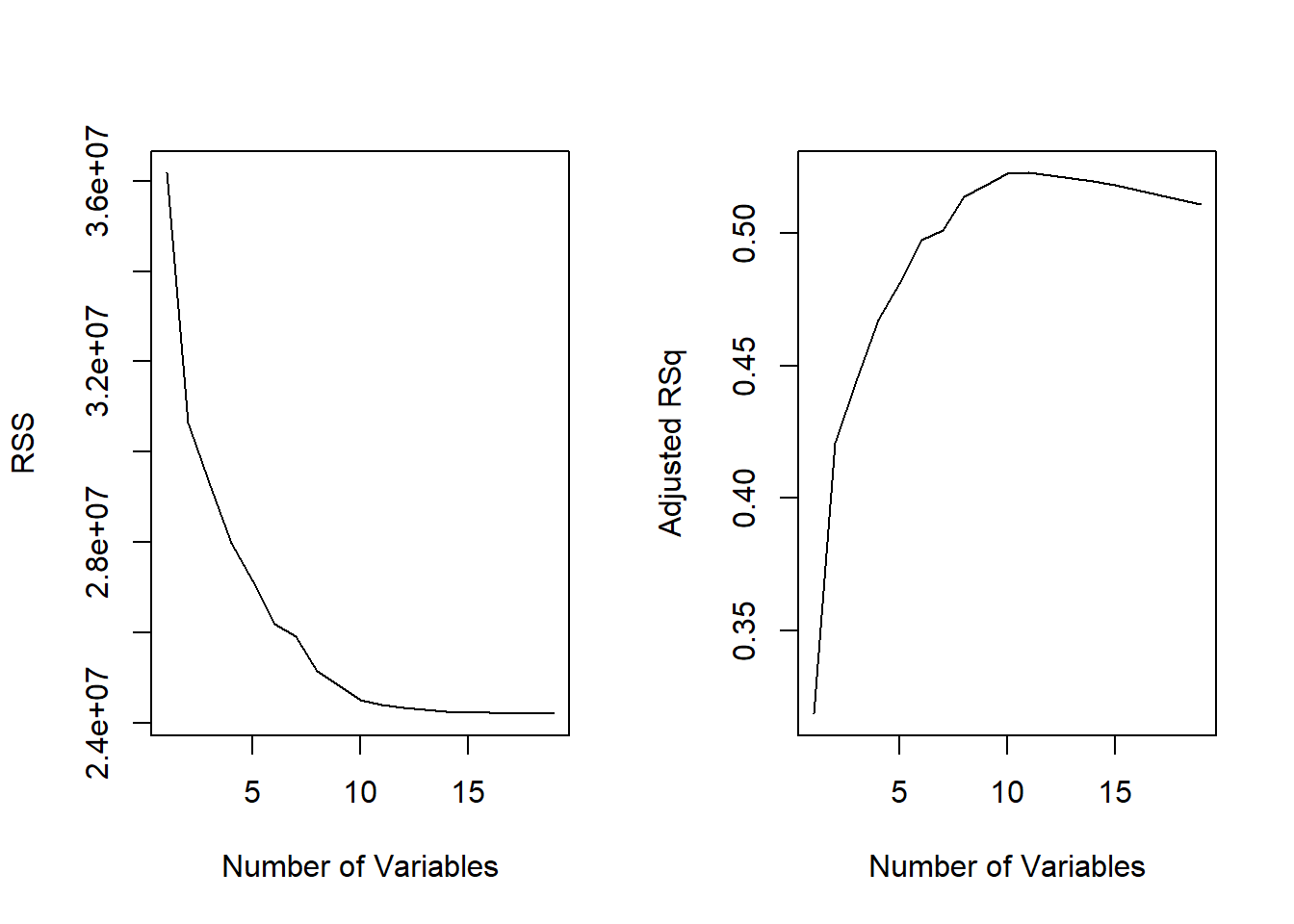
The points() command works like the plot()
command, except that it puts points on a plot that has already been
created, instead of creating a new plot. The which.max()
function can be used to identify the location of the maximum point of a
vector. We will now plot a red dot to indicate the model with the
largest adjusted \(R^2\) statistic.
which.max(reg.summary$adjr2)## [1] 11plot(reg.summary$adjr2, xlab = "Number of Variables", ylab = "Adjusted RSq", type = "l")
points(11, reg.summary$adjr2[11], col = "red", cex = 2, pch = 20)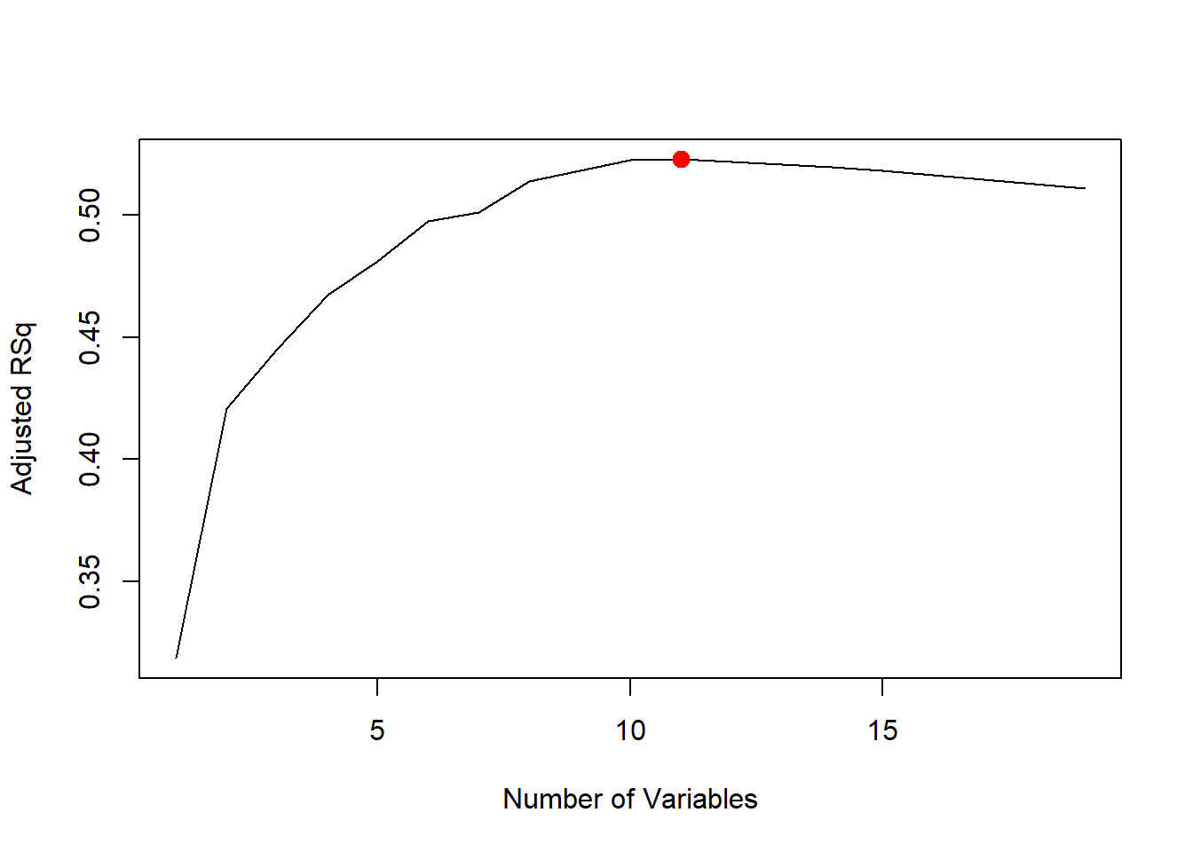
In a similar fashion we can plot the \(C_p\) and BIC statistics, and indicate the
models with the smallest statistic using which.min().
plot(reg.summary$cp, xlab = "Number of Variables", ylab = "Cp", type = "l")
which.min(reg.summary$cp)
## [1] 10points(10, reg.summary$cp[10], col = "red", cex = 2, pch = 20)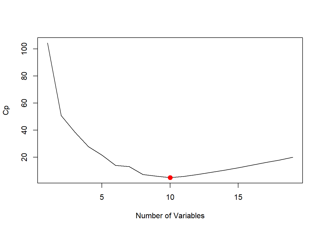
which.min(reg.summary$bic)## [1] 6plot(reg.summary$bic, xlab = "Number of Variables", ylab = "BIC", type = "l")
points(6, reg.summary$bic[6], col = "red", cex = 2, pch = 20)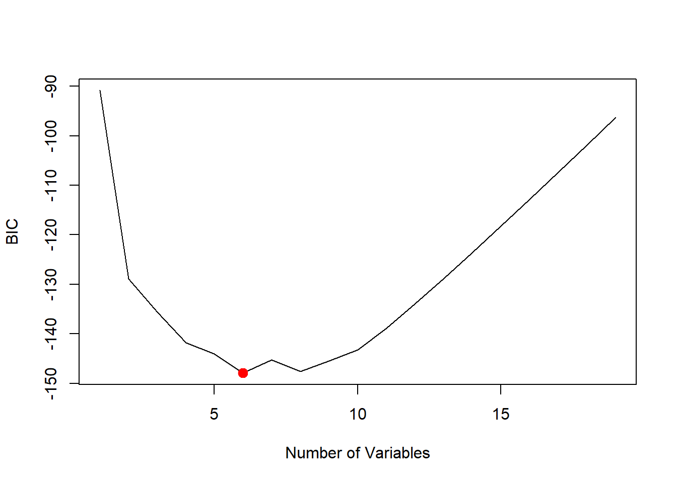
The regsubsets() function has a built-in
plot() command which can be used to display the selected
variables for the best model with a given number of predictors, ranked
according to the BIC, \(C_p\), adjusted
\(R^2\), or AIC. To find out more about
this function, type ?plot.regsubsets.
plot(regfit.full, scale = "r2")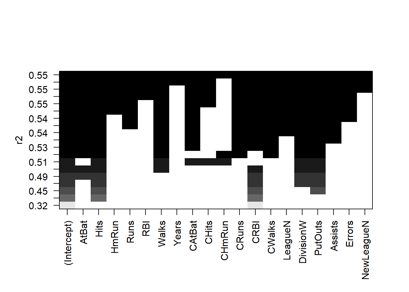
plot(regfit.full, scale = "adjr2")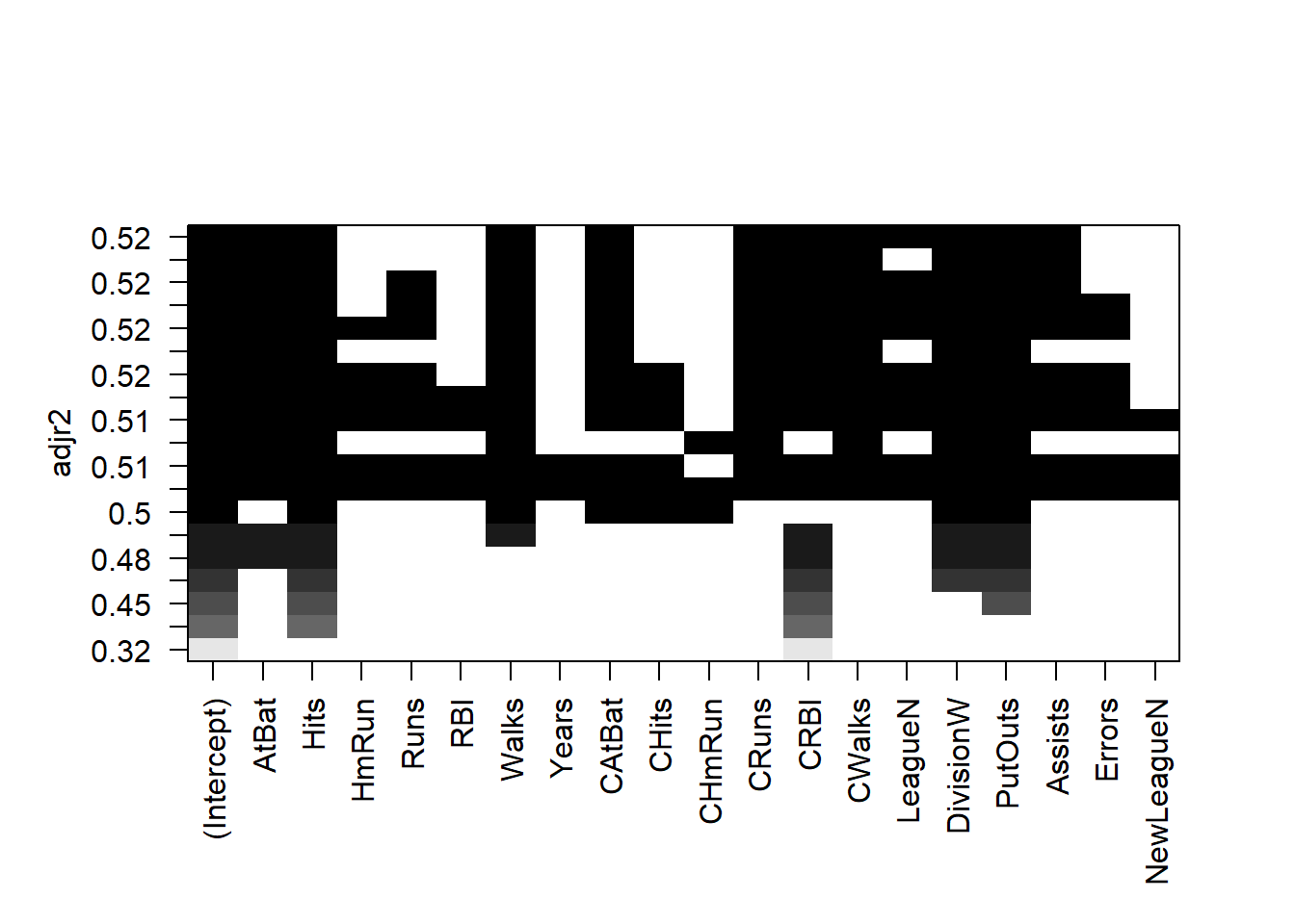
plot(regfit.full, scale = "Cp")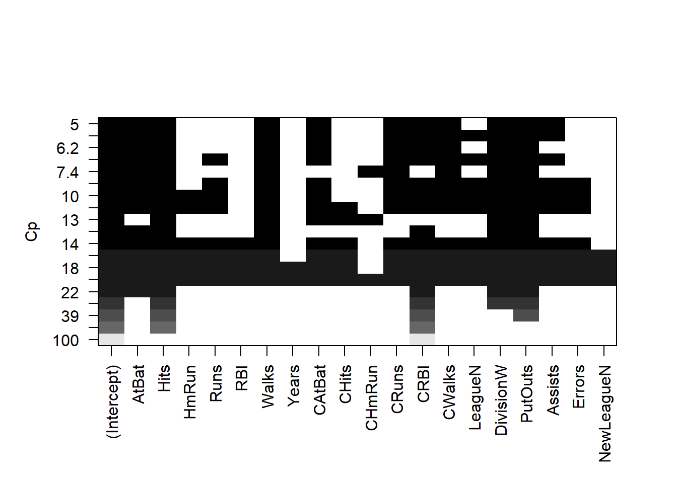
plot(regfit.full, scale = "bic")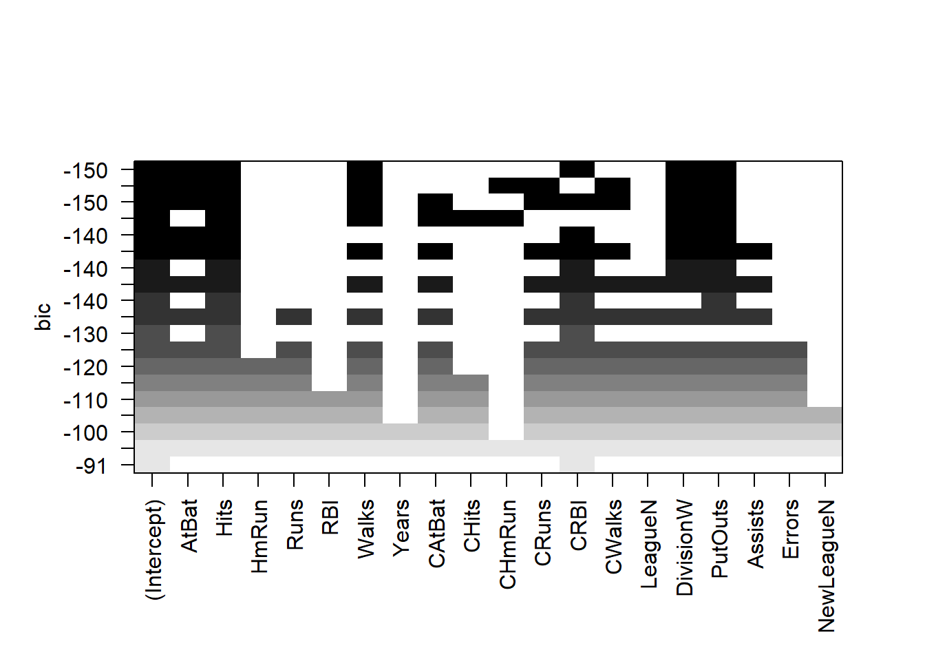
The top row of each plot contains a black square for each variable
selected according to the optimal model associated with that statistic.
For instance, we see that several models share a BIC close to \(-150\). However, the model with the lowest
BIC is the six-variable model that contains only AtBat,
Hits, Walks, CRBI,
DivisionW, and PutOuts.
We can use the coef() function to see the coefficient
estimates associated with this model.
coef(regfit.full, 6)## (Intercept) AtBat Hits Walks CRBI DivisionW
## 91.5117981 -1.8685892 7.6043976 3.6976468 0.6430169 -122.9515338
## PutOuts
## 0.2643076Forward and Backward Stepwise Selection
We can also use the regsubsets() function to perform
forward stepwise or backward stepwise selection, using the argument
method = "forward" or method = "backward".
regfit.fwd <- regsubsets(Salary ~ ., data = Hitters, nvmax = 19, method = "forward")
summary(regfit.fwd)
## Subset selection object
## Call: regsubsets.formula(Salary ~ ., data = Hitters, nvmax = 19, method = "forward")
## 19 Variables (and intercept)
## Forced in Forced out
## AtBat FALSE FALSE
## Hits FALSE FALSE
## HmRun FALSE FALSE
## Runs FALSE FALSE
## RBI FALSE FALSE
## Walks FALSE FALSE
## Years FALSE FALSE
## CAtBat FALSE FALSE
## CHits FALSE FALSE
## CHmRun FALSE FALSE
## CRuns FALSE FALSE
## CRBI FALSE FALSE
## CWalks FALSE FALSE
## LeagueN FALSE FALSE
## DivisionW FALSE FALSE
## PutOuts FALSE FALSE
## Assists FALSE FALSE
## Errors FALSE FALSE
## NewLeagueN FALSE FALSE
## 1 subsets of each size up to 19
## Selection Algorithm: forward
## AtBat Hits HmRun Runs RBI Walks Years CAtBat CHits CHmRun CRuns CRBI
## 1 ( 1 ) " " " " " " " " " " " " " " " " " " " " " " "*"
## 2 ( 1 ) " " "*" " " " " " " " " " " " " " " " " " " "*"
## 3 ( 1 ) " " "*" " " " " " " " " " " " " " " " " " " "*"
## 4 ( 1 ) " " "*" " " " " " " " " " " " " " " " " " " "*"
## 5 ( 1 ) "*" "*" " " " " " " " " " " " " " " " " " " "*"
## 6 ( 1 ) "*" "*" " " " " " " "*" " " " " " " " " " " "*"
## 7 ( 1 ) "*" "*" " " " " " " "*" " " " " " " " " " " "*"
## 8 ( 1 ) "*" "*" " " " " " " "*" " " " " " " " " "*" "*"
## 9 ( 1 ) "*" "*" " " " " " " "*" " " "*" " " " " "*" "*"
## 10 ( 1 ) "*" "*" " " " " " " "*" " " "*" " " " " "*" "*"
## 11 ( 1 ) "*" "*" " " " " " " "*" " " "*" " " " " "*" "*"
## 12 ( 1 ) "*" "*" " " "*" " " "*" " " "*" " " " " "*" "*"
## 13 ( 1 ) "*" "*" " " "*" " " "*" " " "*" " " " " "*" "*"
## 14 ( 1 ) "*" "*" "*" "*" " " "*" " " "*" " " " " "*" "*"
## 15 ( 1 ) "*" "*" "*" "*" " " "*" " " "*" "*" " " "*" "*"
## 16 ( 1 ) "*" "*" "*" "*" "*" "*" " " "*" "*" " " "*" "*"
## 17 ( 1 ) "*" "*" "*" "*" "*" "*" " " "*" "*" " " "*" "*"
## 18 ( 1 ) "*" "*" "*" "*" "*" "*" "*" "*" "*" " " "*" "*"
## 19 ( 1 ) "*" "*" "*" "*" "*" "*" "*" "*" "*" "*" "*" "*"
## CWalks LeagueN DivisionW PutOuts Assists Errors NewLeagueN
## 1 ( 1 ) " " " " " " " " " " " " " "
## 2 ( 1 ) " " " " " " " " " " " " " "
## 3 ( 1 ) " " " " " " "*" " " " " " "
## 4 ( 1 ) " " " " "*" "*" " " " " " "
## 5 ( 1 ) " " " " "*" "*" " " " " " "
## 6 ( 1 ) " " " " "*" "*" " " " " " "
## 7 ( 1 ) "*" " " "*" "*" " " " " " "
## 8 ( 1 ) "*" " " "*" "*" " " " " " "
## 9 ( 1 ) "*" " " "*" "*" " " " " " "
## 10 ( 1 ) "*" " " "*" "*" "*" " " " "
## 11 ( 1 ) "*" "*" "*" "*" "*" " " " "
## 12 ( 1 ) "*" "*" "*" "*" "*" " " " "
## 13 ( 1 ) "*" "*" "*" "*" "*" "*" " "
## 14 ( 1 ) "*" "*" "*" "*" "*" "*" " "
## 15 ( 1 ) "*" "*" "*" "*" "*" "*" " "
## 16 ( 1 ) "*" "*" "*" "*" "*" "*" " "
## 17 ( 1 ) "*" "*" "*" "*" "*" "*" "*"
## 18 ( 1 ) "*" "*" "*" "*" "*" "*" "*"
## 19 ( 1 ) "*" "*" "*" "*" "*" "*" "*"regfit.bwd <- regsubsets(Salary ~ ., data = Hitters, nvmax = 19, method = "backward")
summary(regfit.bwd)## Subset selection object
## Call: regsubsets.formula(Salary ~ ., data = Hitters, nvmax = 19, method = "backward")
## 19 Variables (and intercept)
## Forced in Forced out
## AtBat FALSE FALSE
## Hits FALSE FALSE
## HmRun FALSE FALSE
## Runs FALSE FALSE
## RBI FALSE FALSE
## Walks FALSE FALSE
## Years FALSE FALSE
## CAtBat FALSE FALSE
## CHits FALSE FALSE
## CHmRun FALSE FALSE
## CRuns FALSE FALSE
## CRBI FALSE FALSE
## CWalks FALSE FALSE
## LeagueN FALSE FALSE
## DivisionW FALSE FALSE
## PutOuts FALSE FALSE
## Assists FALSE FALSE
## Errors FALSE FALSE
## NewLeagueN FALSE FALSE
## 1 subsets of each size up to 19
## Selection Algorithm: backward
## AtBat Hits HmRun Runs RBI Walks Years CAtBat CHits CHmRun CRuns CRBI
## 1 ( 1 ) " " " " " " " " " " " " " " " " " " " " "*" " "
## 2 ( 1 ) " " "*" " " " " " " " " " " " " " " " " "*" " "
## 3 ( 1 ) " " "*" " " " " " " " " " " " " " " " " "*" " "
## 4 ( 1 ) "*" "*" " " " " " " " " " " " " " " " " "*" " "
## 5 ( 1 ) "*" "*" " " " " " " "*" " " " " " " " " "*" " "
## 6 ( 1 ) "*" "*" " " " " " " "*" " " " " " " " " "*" " "
## 7 ( 1 ) "*" "*" " " " " " " "*" " " " " " " " " "*" " "
## 8 ( 1 ) "*" "*" " " " " " " "*" " " " " " " " " "*" "*"
## 9 ( 1 ) "*" "*" " " " " " " "*" " " "*" " " " " "*" "*"
## 10 ( 1 ) "*" "*" " " " " " " "*" " " "*" " " " " "*" "*"
## 11 ( 1 ) "*" "*" " " " " " " "*" " " "*" " " " " "*" "*"
## 12 ( 1 ) "*" "*" " " "*" " " "*" " " "*" " " " " "*" "*"
## 13 ( 1 ) "*" "*" " " "*" " " "*" " " "*" " " " " "*" "*"
## 14 ( 1 ) "*" "*" "*" "*" " " "*" " " "*" " " " " "*" "*"
## 15 ( 1 ) "*" "*" "*" "*" " " "*" " " "*" "*" " " "*" "*"
## 16 ( 1 ) "*" "*" "*" "*" "*" "*" " " "*" "*" " " "*" "*"
## 17 ( 1 ) "*" "*" "*" "*" "*" "*" " " "*" "*" " " "*" "*"
## 18 ( 1 ) "*" "*" "*" "*" "*" "*" "*" "*" "*" " " "*" "*"
## 19 ( 1 ) "*" "*" "*" "*" "*" "*" "*" "*" "*" "*" "*" "*"
## CWalks LeagueN DivisionW PutOuts Assists Errors NewLeagueN
## 1 ( 1 ) " " " " " " " " " " " " " "
## 2 ( 1 ) " " " " " " " " " " " " " "
## 3 ( 1 ) " " " " " " "*" " " " " " "
## 4 ( 1 ) " " " " " " "*" " " " " " "
## 5 ( 1 ) " " " " " " "*" " " " " " "
## 6 ( 1 ) " " " " "*" "*" " " " " " "
## 7 ( 1 ) "*" " " "*" "*" " " " " " "
## 8 ( 1 ) "*" " " "*" "*" " " " " " "
## 9 ( 1 ) "*" " " "*" "*" " " " " " "
## 10 ( 1 ) "*" " " "*" "*" "*" " " " "
## 11 ( 1 ) "*" "*" "*" "*" "*" " " " "
## 12 ( 1 ) "*" "*" "*" "*" "*" " " " "
## 13 ( 1 ) "*" "*" "*" "*" "*" "*" " "
## 14 ( 1 ) "*" "*" "*" "*" "*" "*" " "
## 15 ( 1 ) "*" "*" "*" "*" "*" "*" " "
## 16 ( 1 ) "*" "*" "*" "*" "*" "*" " "
## 17 ( 1 ) "*" "*" "*" "*" "*" "*" "*"
## 18 ( 1 ) "*" "*" "*" "*" "*" "*" "*"
## 19 ( 1 ) "*" "*" "*" "*" "*" "*" "*"For instance, we see that using forward stepwise selection, the best
one-variable model contains only CRBI, and the best
two-variable model additionally includes Hits. For this
data, the best one-variable through six-variable models are each
identical for best subset and forward selection. However, the best
seven-variable models identified by forward stepwise selection, backward
stepwise selection, and best subset selection are different.
coef(regfit.full, 7)## (Intercept) Hits Walks CAtBat CHits CHmRun
## 79.4509472 1.2833513 3.2274264 -0.3752350 1.4957073 1.4420538
## DivisionW PutOuts
## -129.9866432 0.2366813coef(regfit.fwd, 7)## (Intercept) AtBat Hits Walks CRBI CWalks
## 109.7873062 -1.9588851 7.4498772 4.9131401 0.8537622 -0.3053070
## DivisionW PutOuts
## -127.1223928 0.2533404coef(regfit.bwd, 7)## (Intercept) AtBat Hits Walks CRuns CWalks
## 105.6487488 -1.9762838 6.7574914 6.0558691 1.1293095 -0.7163346
## DivisionW PutOuts
## -116.1692169 0.3028847Choosing Among Models Using the Validation-Set Approach and Cross-Validation
We just saw that it is possible to choose among a set of models of different sizes using \(C_p\), BIC, and adjusted \(R^2\). We will now consider how to do this using the validation set and cross-validation approaches.
In order for these approaches to yield accurate estimates of the test error, we must use only the training observations to perform all aspects of model-fitting—including variable selection. Therefore, the determination of which model of a given size is best must be made using only the training observations. This point is subtle but important.
If the full data set is used to perform the best subset selection step, the validation set errors and cross-validation errors that we obtain will not be accurate estimates of the test error.
In order to use the validation set approach, we begin by splitting
the observations into a training set and a test set. We do this by
creating a random vector, train, of elements equal to
TRUE if the corresponding observation is in the training
set, and FALSE otherwise. The vector test has
a TRUE if the observation is in the test set, and a
FALSE otherwise. Note the ! in the command to
create test causes TRUEs to be switched to
FALSEs and vice versa. We also set a random seed so that
the user will obtain the same training set/test set split.
set.seed(1)
train <- sample(c(TRUE, FALSE), nrow(Hitters), replace = TRUE)
test <- (!train)
Now, we apply regsubsets() to the training set in order
to perform best subset selection.
regfit.best <- regsubsets(Salary ~ ., data = Hitters[train, ], nvmax = 19)Notice that we subset the Hitters data frame directly in
the call in order to access only the training subset of the data, using
the expression Hitters[train, ]. We now compute the
validation set error for the best model of each model size. We first
make a model matrix from the test data.
test.mat <- model.matrix(Salary ~ ., data = Hitters[test, ])The model.matrix() function is used in many regression
packages for building an “X” matrix from data. Now we run a loop, and
for each size i, we extract the coefficients from
regfit.best for the best model of that size, multiply them
into the appropriate columns of the test model matrix to form the
predictions, and compute the test MSE.
val.errors <- rep(NA, 19)
for (i in 1:19) {
 coefi <- coef(regfit.best, id = i)
 pred <- test.mat[, names(coefi)] %*% coefi
 val.errors[i] <- mean((Hitters$Salary[test] - pred)^2)
}
We find that the best model is the one that contains seven variables.
val.errors## [1] 164377.3 144405.5 152175.7 145198.4 137902.1 139175.7 126849.0 136191.4
## [9] 132889.6 135434.9 136963.3 140694.9 140690.9 141951.2 141508.2 142164.4
## [17] 141767.4 142339.6 142238.2which.min(val.errors)## [1] 7coef(regfit.best, 7)## (Intercept) AtBat Hits Walks CRuns CWalks
## 67.1085369 -2.1462987 7.0149547 8.0716640 1.2425113 -0.8337844
## DivisionW PutOuts
## -118.4364998 0.2526925This was a little tedious, partly because there is no
predict() method for regsubsets(). Since we
will be using this function again, we can capture our steps above and
write our own predict method.
 predict.regsubsets <- function(object, newdata, id, ...) {
  form <- as.formula(object$call[[2]])
  mat <- model.matrix(form, newdata)
  coefi <- coef(object, id = id)
  xvars <- names(coefi)
  mat[, xvars] %*% coefi
 }
Our function pretty much mimics what we did above. The only complex
part is how we extracted the formula used in the call to
regsubsets(). We demonstrate how we use this function
below, when we do cross-validation.
Finally, we perform best subset selection on the full data set, and select the best seven-variable model. It is important that we make use of the full data set in order to obtain more accurate coefficient estimates. Note that we perform best subset selection on the full data set and select the best seven-variable model, rather than simply using the variables that were obtained from the training set, because the best seven-variable model on the full data set may differ from the corresponding model on the training set.
regfit.best <- regsubsets(Salary ~ ., data = Hitters, nvmax = 19)
coef(regfit.best, 7)
## (Intercept) Hits Walks CAtBat CHits CHmRun
## 79.4509472 1.2833513 3.2274264 -0.3752350 1.4957073 1.4420538
## DivisionW PutOuts
## -129.9866432 0.2366813In fact, we see that the best seven-variable model on the full data set has a different set of variables than the best seven-variable model on the training set.
We now try to choose among the models of different sizes using
cross-validation. This approach is somewhat involved, as we must perform
best subset selection within each of the \(k\) training sets. Despite this, we
see that with its clever subsetting syntax, R makes this
job quite easy. First, we create a vector that allocates each
observation to one of \(k=10\) folds,
and we create a matrix in which we will store the results.
k <- 10
n <- nrow(Hitters)
set.seed(1)
folds <- sample(rep(1:k, length = n))
cv.errors <- matrix(NA, k, 19, dimnames = list(NULL, paste(1:19)))
Now we write a for loop that performs cross-validation. In the \(j\)th fold, the elements of
folds that equal j are in the test set, and
the remainder are in the training set. We make our predictions for each
model size (using our new predict() method), compute the
test errors on the appropriate subset, and store them in the appropriate
slot in the matrix cv.errors. Note that in the following
code R will automatically use our
predict.regsubsets() function when we call
predict() because the best.fit object has
class regsubsets.
for (j in 1:k) {
  best.fit <- regsubsets(Salary ~ ., data = Hitters[folds != j, ], nvmax = 19)
  for (i in 1:19) {
    pred <- predict(best.fit, Hitters[folds == j, ], id = i)
    cv.errors[j, i] <- mean((Hitters$Salary[folds == j] - pred)^2)
   }
 }
This has given us a \(10 \times 19\)
matrix, of which the \((j,i)\)th
element corresponds to the test MSE for the \(j\)th cross-validation fold for the best
\(i\)-variable model. We use the
apply() function to average over the columns of this matrix
in order to obtain a vector for which the \(i\)th element is the cross-validation error
for the \(i\)-variable model.
mean.cv.errors <- apply(cv.errors, 2, mean)
mean.cv.errors
## 1 2 3 4 5 6 7 8
## 143439.8 126817.0 134214.2 131782.9 130765.6 120382.9 121443.1 114363.7
## 9 10 11 12 13 14 15 16
## 115163.1 109366.0 112738.5 113616.5 115557.6 115853.3 115630.6 116050.0
## 17 18 19
## 116117.0 116419.3 116299.1par(mfrow = c(1, 1))
plot(mean.cv.errors, type = "b")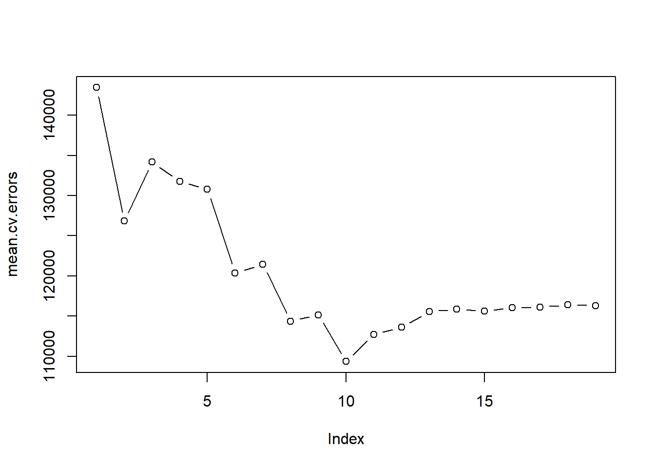
We see that cross-validation selects a 10-variable model. We now perform best subset selection on the full data set in order to obtain the 10-variable model.
reg.best <- regsubsets(Salary ~ ., data = Hitters, nvmax = 19)
coef(reg.best, 10)
## (Intercept) AtBat Hits Walks CAtBat CRuns
## 162.5354420 -2.1686501 6.9180175 5.7732246 -0.1300798 1.4082490
## CRBI CWalks DivisionW PutOuts Assists
## 0.7743122 -0.8308264 -112.3800575 0.2973726 0.2831680