Supervised Learning III - Logistic Regression
Patrick PUN Chi Seng (NTU Sg)
References
Chapters 4.7.2 [ISLR2] An Introduction to Statistical Learning - with Applications in R (2nd Edition). Free access to download the book: https://www.statlearning.com/
To see the help file of a function funcname, type
?funcname.
Logistic Regression
We use again the stock market data for illustration; see lab notes
for Supervised Learning I for the exploratory data analysis. We will fit
a logistic regression model in order to predict direction
using lagone through lagfive and
volume.
library(ISLR2)
attach(Smarket)
The glm() function can be used to fit many types of
generalized linear models, including logistic regression. The syntax of
the glm() function is similar to that of lm(),
except that we must pass in the argument family = binomial
in order to tell R to run a logistic regression rather than
some other type of generalized linear model.
glm.fits <- glm(
    Direction ~ Lag1 + Lag2 + Lag3 + Lag4 + Lag5 + Volume,
    data = Smarket, family = binomial
  )
summary(glm.fits)
##
## Call:
## glm(formula = Direction ~ Lag1 + Lag2 + Lag3 + Lag4 + Lag5 +
## Volume, family = binomial, data = Smarket)
##
## Coefficients:
## Estimate Std. Error z value Pr(>|z|)
## (Intercept) -0.126000 0.240736 -0.523 0.601
## Lag1 -0.073074 0.050167 -1.457 0.145
## Lag2 -0.042301 0.050086 -0.845 0.398
## Lag3 0.011085 0.049939 0.222 0.824
## Lag4 0.009359 0.049974 0.187 0.851
## Lag5 0.010313 0.049511 0.208 0.835
## Volume 0.135441 0.158360 0.855 0.392
##
## (Dispersion parameter for binomial family taken to be 1)
##
## Null deviance: 1731.2 on 1249 degrees of freedom
## Residual deviance: 1727.6 on 1243 degrees of freedom
## AIC: 1741.6
##
## Number of Fisher Scoring iterations: 3The smallest p-value here is associated with lagone. The
negative coefficient for this predictor suggests that if the market had
a positive return yesterday, then it is less likely to go up today.
However, at a value of 0.15, the p-value is still relatively large, and
so there is no clear evidence of a real association between
lagone and direction.
We use the coef() function in order to access just the
coefficients for this fitted model. We can also use the
summary() function to access particular aspects of the
fitted model, such as the \(p\)-values
for the coefficients.
coef(glm.fits)## (Intercept) Lag1 Lag2 Lag3 Lag4 Lag5
## -0.126000257 -0.073073746 -0.042301344 0.011085108 0.009358938 0.010313068
## Volume
## 0.135440659summary(glm.fits)$coef## Estimate Std. Error z value Pr(>|z|)
## (Intercept) -0.126000257 0.24073574 -0.5233966 0.6006983
## Lag1 -0.073073746 0.05016739 -1.4565986 0.1452272
## Lag2 -0.042301344 0.05008605 -0.8445733 0.3983491
## Lag3 0.011085108 0.04993854 0.2219750 0.8243333
## Lag4 0.009358938 0.04997413 0.1872757 0.8514445
## Lag5 0.010313068 0.04951146 0.2082966 0.8349974
## Volume 0.135440659 0.15835970 0.8552723 0.3924004summary(glm.fits)$coef[, 4]## (Intercept) Lag1 Lag2 Lag3 Lag4 Lag5
## 0.6006983 0.1452272 0.3983491 0.8243333 0.8514445 0.8349974
## Volume
## 0.3924004The predict() function can be used to predict the
probability that the market will go up, given values of the predictors.
The type = "response" option tells R to output
probabilities of the form \(\mathbb{P}(Y=1|X)\), as opposed to other
information such as the logit. If no data set is supplied to the
predict() function, then the probabilities are computed for
the training data that was used to fit the logistic regression model.
Here we have printed only the first ten probabilities. We know that
these values correspond to the probability of the market going up,
rather than down, because the contrasts() function
indicates that R has created a dummy variable with a 1 for
Up.
glm.probs <- predict(glm.fits, type = "response")
glm.probs[1:10]
## 1 2 3 4 5 6 7 8
## 0.5070841 0.4814679 0.4811388 0.5152224 0.5107812 0.5069565 0.4926509 0.5092292
## 9 10
## 0.5176135 0.4888378contrasts(Direction)## Up
## Down 0
## Up 1In order to make a prediction as to whether the market will go up or
down on a particular day, we must convert these predicted probabilities
into class labels, Up or Down. The following
two commands create a vector of class predictions based on whether the
predicted probability of a market increase is greater than or less than
0.5.
glm.pred <- rep("Down", 1250)
glm.pred[glm.probs > .5] = "Up"
The first command creates a vector of 1,250 Down
elements. The second line transforms to Up all of the
elements for which the predicted probability of a market increase
exceeds 0.5. Given these predictions, the table() function
can be used to produce a confusion matrix in order to determine how many
observations were correctly or incorrectly classified.
ConfusionMatrix = table(glm.pred, Direction); ConfusionMatrix## Direction
## glm.pred Down Up
## Down 145 141
## Up 457 507sum(diag(ConfusionMatrix)) / sum(ConfusionMatrix)## [1] 0.5216mean(glm.pred == Direction)## [1] 0.5216The diagonal elements of the confusion matrix indicate correct
predictions, while the off-diagonals represent incorrect predictions.
Hence our model correctly predicted that the market would go up on 507
days and that it would go down on 145 days, for a total of 507+145 = 652
correct predictions. The mean() function can be used to
compute the fraction of days for which the prediction was correct. In
this case, logistic regression correctly predicted the movement of the
market 52.2% of the time.
At first glance, it appears that the logistic regression model is working a little better than random guessing. However, this result is misleading because we trained and tested the model on the same set of 1,250 observations. In other words, 100%-52.2%=47.8%, is the training error rate. As we have seen previously, the training error rate is often overly optimistic—it tends to underestimate the test error rate. In order to better assess the accuracy of the logistic regression model in this setting, we can fit the model using part of the data, and then examine how well it predicts the held out data. This will yield a more realistic error rate, in the sense that in practice we will be interested in our model’s performance not on the data that we used to fit the model, but rather on days in the future for which the market’s movements are unknown.
To implement this strategy, we will first create a vector corresponding to the observations from 2001 through 2004. We will then use this vector to create a held out data set of observations from 2005.
train <- (Year < 2005)
Smarket.2005 <- Smarket[!train, ]
dim(Smarket.2005)
## [1] 252 9Direction.2005 <- Direction[!train]The object train is a vector of 1,250 elements,
corresponding to the observations in our data set. The elements of the
vector that correspond to observations that occurred before 2005 are set
to TRUE, whereas those that correspond to observations in
2005 are set to FALSE. The object train is a
Boolean vector, since its elements are TRUE and
FALSE. Boolean vectors can be used to obtain a subset of
the rows or columns of a matrix. For instance, the command
Smarket[train, ] would pick out a submatrix of the stock
market data set, corresponding only to the dates before 2005, since
those are the ones for which the elements of train are
TRUE. The ! symbol can be used to reverse all
of the elements of a Boolean vector. That is, !train is a
vector similar to train, except that the elements that are
TRUE in train get swapped to
FALSE in !train, and the elements that are
FALSE in train get swapped to
TRUE in !train. Therefore,
Smarket[!train, ] yields a submatrix of the stock market
data containing only the observations for which train is
FALSE—that is, the observations with dates in 2005. The
output above indicates that there are 252 such observations.
We now fit a logistic regression model using only the subset of the
observations that correspond to dates before 2005, using the
subset argument. We then obtain predicted probabilities of
the stock market going up for each of the days in our test set—that is,
for the days in 2005.
glm.fits <- glm(
    Direction ~ Lag1 + Lag2 + Lag3 + Lag4 + Lag5 + Volume,
    data = Smarket, family = binomial, subset = train
  )
glm.probs <- predict(glm.fits, Smarket.2005,
    type = "response")
Notice that we have trained and tested our model on two completely separate data sets: training was performed using only the dates before 2005, and testing was performed using only the dates in 2005. Finally, we compute the predictions for 2005 and compare them to the actual movements of the market over that time period.
glm.pred <- rep("Down", 252)
glm.pred[glm.probs > .5] <- "Up"
table(glm.pred, Direction.2005)
## Direction.2005
## glm.pred Down Up
## Down 77 97
## Up 34 44mean(glm.pred == Direction.2005)## [1] 0.4801587mean(glm.pred != Direction.2005)## [1] 0.5198413The != notation means not equal to, and so the
last command computes the test set error rate. The results are rather
disappointing: the test error rate is 52%, which is worse than random
guessing! Of course this result is not all that surprising, given that
one would not generally expect to be able to use previous days’ returns
to predict future market performance. (After all, if it were possible to
do so, then the authors of this book would be out striking it rich
rather than writing a statistics textbook.)
We recall that the logistic regression model had very underwhelming
p-values associated with all of the predictors, and that the smallest
p-value, though not very small, corresponded to lagone.
Perhaps by removing the variables that appear not to be helpful in
predicting direction, we can obtain a more effective model.
After all, using predictors that have no relationship with the response
tends to cause a deterioration in the test error rate (since such
predictors cause an increase in variance without a corresponding
decrease in bias), and so removing such predictors may in turn yield an
improvement.
Below we have refit the logistic regression using just
lagone and lagtwo, which seemed to have the
highest predictive power in the original logistic regression model.
glm.fits <- glm(Direction ~ Lag1 + Lag2, data = Smarket, family = binomial, subset = train)
glm.probs <- predict(glm.fits, Smarket.2005, type = "response")
glm.pred <- rep("Down", 252)
glm.pred[glm.probs > .5] <- "Up"
table(glm.pred, Direction.2005)
## Direction.2005
## glm.pred Down Up
## Down 35 35
## Up 76 106mean(glm.pred == Direction.2005)## [1] 0.5595238precision = 106 / (106 + 76); precision## [1] 0.5824176Now the results appear to be a little better: \(56\%\) of the daily movements have been correctly predicted. It is worth noting that in this case, a much simpler strategy of predicting that the market will increase every day will also be correct \(56\%\) of the time! Hence, in terms of overall error rate, the logistic regression method is no better than the naive approach. However, the confusion matrix shows that on days when logistic regression predicts an increase in the market, it has a \(58\%\) accuracy rate. This suggests a possible trading strategy of buying on days when the model predicts an increasing market, and avoiding trades on days when a decrease is predicted. Of course one would need to investigate more carefully whether this small improvement was real or just due to random chance.
Suppose that we want to predict the returns associated with
particular values of lagone and lagtwo. In
particular, we want to predict direction on a day when
lagone and lagtwo equal 1.2 and 1.1,
respectively, and on a day when they equal 1.5 and -0.8. We do this
using the predict() function.
predict(glm.fits,
    newdata = data.frame(Lag1 = c(1.2, 1.5),  Lag2 = c(1.1, -0.8)),
    type = "response"
  )
## 1 2
## 0.4791462 0.4960939Regularized Logistic Regression (Ridge & Lasso)
We extend logistic regression with \(\ell_2\) (ridge) and \(\ell_1\) (lasso) penalties using
glmnet. Standardization matters for
penalized models; glmnet() standardizes predictors
by default. If you manually scale features, use
training-set statistics only to avoid leakage.
We predict Direction (Up/Down) from
Lag1–Lag5 and Volume using the
same train/test split as before (train:
Year < 2005; test: 2005). We select the tuning parameter
\(\lambda\) by
cross-validation.
library(glmnet)## Loading required package: Matrix## Loaded glmnet 4.1-10# Design matrix (drop intercept) and response
x <- model.matrix(Direction ~ Lag1 + Lag2 + Lag3 + Lag4 + Lag5 + Volume, data = Smarket)[, -1]
y <- Smarket$Direction
# Train/test split (consistent with earlier section)
train <- (Smarket$Year < 2005)
test_idx <- which(!train)
y_test <- y[test_idx]Ridge-penalized Logistic Regression (\(\alpha=0\)) with CV
set.seed(1)
cv.ridge <- cv.glmnet(x[train, ], y[train], family = "binomial", alpha = 0)  # 10-fold CV by default
plot(cv.ridge)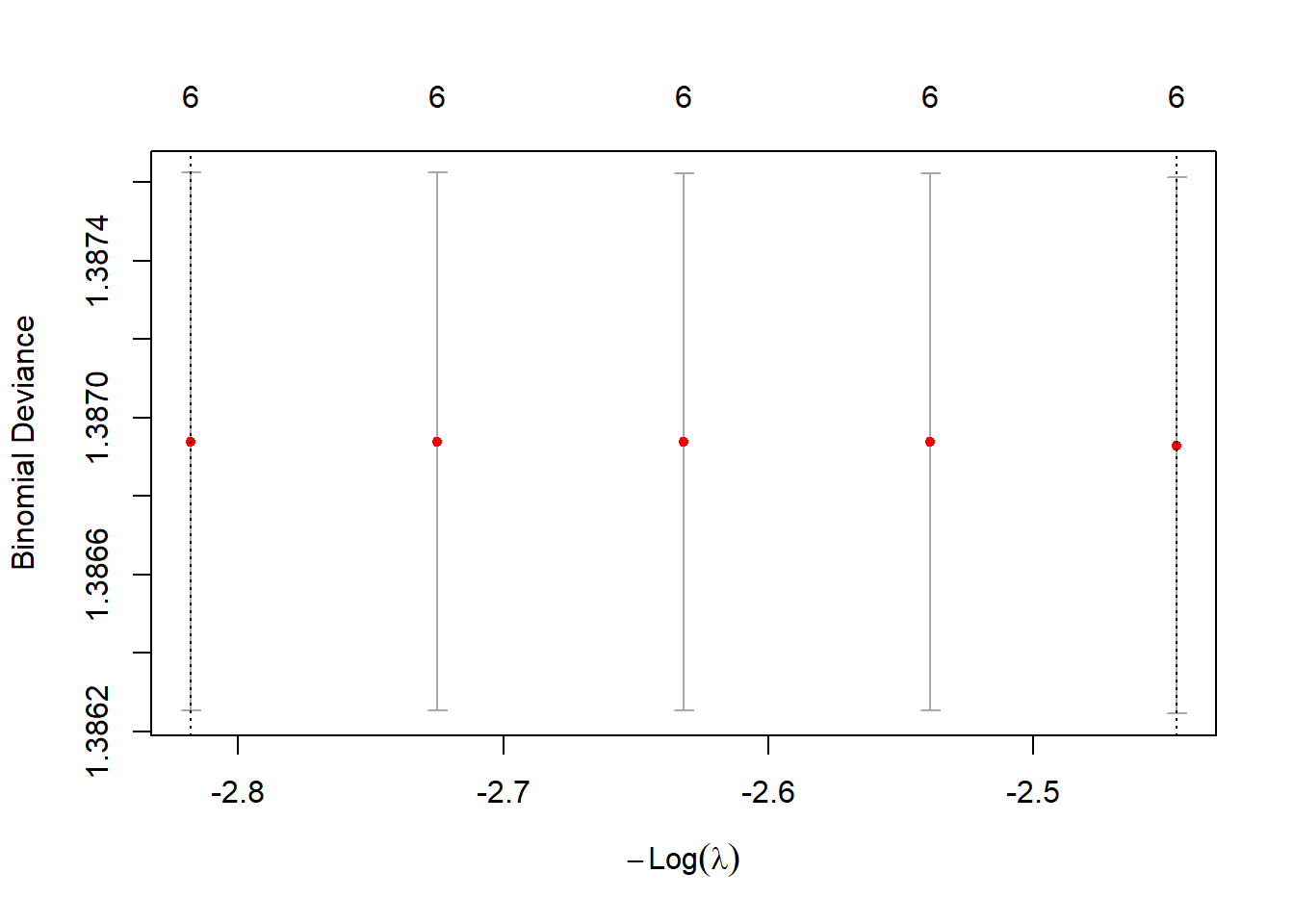
bestlam_ridge <- cv.ridge$lambda.min; bestlam_ridge## [1] 11.54079# Predict class labels on 2005 data
ridge.class <- predict(cv.ridge, s = bestlam_ridge, newx = x[test_idx, ], type = "class")
table(ridge.class, y_test)## y_test
## ridge.class Down Up
## Up 111 141mean(ridge.class == y_test)## [1] 0.5595238# Inspect selected (nonzero) coefficients under Ridge
predict(cv.ridge$glmnet.fit, s = bestlam_ridge, type = "coefficients")## 7 x 1 sparse Matrix of class "dgCMatrix"
## s=11.54079
## (Intercept) 3.556275e-02
## Lag1 -1.155157e-03
## Lag2 -9.162571e-04
## Lag3 2.171575e-04
## Lag4 1.903505e-04
## Lag5 -6.929241e-05
## Volume -2.554238e-03Lasso-penalized Logistic Regression (\(\alpha=1\)) with CV
set.seed(1)
cv.lasso <- cv.glmnet(x[train, ], y[train], family = "binomial", alpha = 1)
plot(cv.lasso)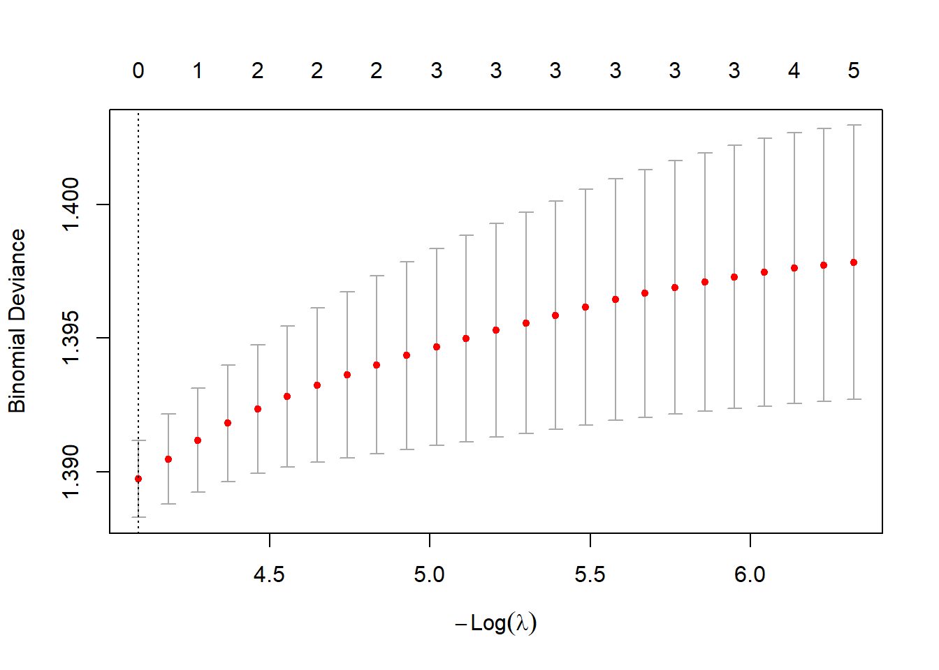
bestlam_lasso <- cv.lasso$lambda.min; bestlam_lasso## [1] 0.01674372# Predict class labels on 2005 data
lasso.class <- predict(cv.lasso, s = bestlam_lasso, newx = x[test_idx, ], type = "class")
table(lasso.class, y_test)## y_test
## lasso.class Down Up
## Up 111 141mean(lasso.class == y_test)## [1] 0.5595238# Inspect selected (nonzero) coefficients under lasso
predict(cv.lasso$glmnet.fit, s = bestlam_lasso, type = "coefficients")## 7 x 1 sparse Matrix of class "dgCMatrix"
## s=0.01674372
## (Intercept) 0.03206688
## Lag1 .
## Lag2 .
## Lag3 .
## Lag4 .
## Lag5 .
## Volume .Platt Scaling for Probability Calibration
Logistic regression already outputs probabilities, but regularized models or other classifiers (e.g., SVM, KNN, random forest) may produce poorly calibrated scores.
Platt scaling is a post-processing step that fits a logistic regression to map raw classifier scores into calibrated probabilities.
Here we illustrate Platt scaling on the ridge-penalized logistic regression fitted earlier. We first obtain the raw predicted probabilities, then fit a calibration model on a held-out validation set.
# Split training set further into "inner-train" and "validation" for calibration
set.seed(1)
train_idx <- which(train)
val_idx <- sample(train_idx, length(train_idx) * 0.3)   # 30% for calibration
inner_train_idx <- setdiff(train_idx, val_idx)

# Refit ridge on inner-train only
cv.ridge.inner <- cv.glmnet(x[inner_train_idx, ], y[inner_train_idx], family = "binomial", alpha = 0)

# Get raw predicted probs on validation set
ridge.prob.val <- predict(cv.ridge.inner, s = "lambda.min", newx = x[val_idx, ], type = "response")

# Fit Platt scaling: logistic regression of true labels on raw scores
platt.model <- glm(y[val_idx] ~ ridge.prob.val, family = binomial)

summary(platt.model)
##
## Call:
## glm(formula = y[val_idx] ~ ridge.prob.val, family = binomial)
##
## Coefficients: (1 not defined because of singularities)
## Estimate Std. Error z value Pr(>|z|)
## (Intercept) -0.04683 0.11569 -0.405 0.686
## ridge.prob.val NA NA NA NA
##
## (Dispersion parameter for binomial family taken to be 1)
##
## Null deviance: 414.34 on 298 degrees of freedom
## Residual deviance: 414.34 on 298 degrees of freedom
## AIC: 416.34
##
## Number of Fisher Scoring iterations: 3Now apply the Platt-calibrated model to new test data. We first get raw ridge probabilities, then pass them through the calibration model:
# Raw ridge probabilities on 2005 test data
ridge.prob.test <- predict(cv.ridge.inner, s = "lambda.min", newx = x[test_idx, ], type = "response")

# Calibrated probabilities via Platt scaling
ridge.prob.calibrated <- predict(platt.model, newdata = data.frame(ridge.prob.val = ridge.prob.test), type = "response")
## Warning: 'newdata' had 252 rows but variables found have 299 rows# Compare calibrated vs uncalibrated predictions
head(cbind(raw = ridge.prob.test, calibrated = ridge.prob.calibrated))## Warning in cbind(raw = ridge.prob.test, calibrated = ridge.prob.calibrated):
## number of rows of result is not a multiple of vector length (arg 2)## lambda.min calibrated
## 999 0.5164521 0.4882943
## 1000 0.5164521 0.4882943
## 1001 0.5164521 0.4882943
## 1002 0.5164521 0.4882943
## 1003 0.5164521 0.4882943
## 1004 0.5164521 0.4882943Multinomial Logistic Regression for Multi-class Classification
We illustrate multinomial (multi-class) logistic
regression using the Iris data. The response
Species has three classes (setosa,
versicolor, virginica). We first fit an
unregularized multinomial model with nnet::multinom, then
show regularized multinomial regression with
glmnet (ridge and lasso) using cross-validation for \(\lambda\).
Reminder: Penalized models are sensitive to feature scale;
glmnet() standardizes by default (use
training stats only if you standardize manually).
# data(iris)
# head(iris)
# summary(iris)
# dim(iris)
# str(iris)
attach(iris)
set.seed(1)
train <- sample(nrow(iris), 0.7*nrow(iris))
iris.train <- iris[train, ]
iris.test <- iris[-train, ]We can’’’t use glm() for multi-class logistic
regression, so we use multinom from nnet.
library(nnet)
nn.fit3 <- multinom(Species ~ ., data = iris.train)
## # weights: 18 (10 variable)
## initial value 115.354290
## iter 10 value 11.843953
## iter 20 value 4.770225
## iter 30 value 4.634061
## iter 40 value 4.621675
## iter 50 value 4.610482
## iter 60 value 4.599042
## iter 70 value 4.588547
## iter 80 value 4.587429
## iter 90 value 4.586110
## iter 100 value 4.585787
## final value 4.585787
## stopped after 100 iterationssummary(nn.fit3) # where are the coefficients for 'setosa'?## Call:
## multinom(formula = Species ~ ., data = iris.train)
##
## Coefficients:
## (Intercept) Sepal.Length Sepal.Width Petal.Length Petal.Width
## versicolor 24.71382 -6.955943 -6.929103 12.19530 -1.618096
## virginica -29.22868 -7.047290 -14.299271 21.96416 14.428062
##
## Std. Errors:
## (Intercept) Sepal.Length Sepal.Width Petal.Length Petal.Width
## versicolor 94.81842 55.35526 89.45746 65.02356 174.5397
## virginica 97.32410 55.33436 89.64671 65.76696 174.5348
##
## Residual Deviance: 9.171573
## AIC: 29.17157Predicted class probabilities, class labels, and confusion matrix:
nn.prob3 <- predict(nn.fit3, type = "probs" , newdata = iris.test)
nn.prob3[1:10,]
## setosa versicolor virginica
## 3 0.9999996 4.464304e-07 5.044485e-34
## 4 0.9999795 2.051327e-05 3.448736e-31
## 5 1.0000000 1.173281e-08 1.796762e-36
## 8 0.9999998 1.588149e-07 2.820985e-34
## 9 0.9999026 9.736580e-05 2.740780e-30
## 11 1.0000000 1.229529e-09 2.307452e-37
## 16 1.0000000 8.638226e-13 2.244358e-41
## 27 0.9999996 3.890274e-07 4.544618e-32
## 30 0.9999827 1.732413e-05 3.668455e-31
## 36 1.0000000 1.636216e-08 6.772453e-36nn.pred3 <- predict(nn.fit3, type = "class" , newdata = iris.test)
nn.pred3[1:10]## [1] setosa setosa setosa setosa setosa setosa setosa setosa setosa setosa
## Levels: setosa versicolor virginicatable(nn.pred3, iris.test$Species) # confusion matrix##
## nn.pred3 setosa versicolor virginica
## setosa 15 0 0
## versicolor 0 17 2
## virginica 0 0 11Regularized Multinomial Logistic Regression (Ridge & Lasso via glmnet)
Below we fit ridge (\(\alpha=0\))
and lasso (\(\alpha=1\)) multinomial
logistic regression with 10-fold CV to choose \(\lambda\), using the same train/test split
as above. glmnet() standardizes predictors by default,
which is recommended for penalties.
library(glmnet)

# Design matrix (drop intercept) and response as factor
x <- model.matrix(Species ~ ., data = iris)[, -1]
y <- iris$Species

# Train/test indices consistent with earlier split
tr_idx <- train
te_idx <- setdiff(seq_len(nrow(iris)), train)
Ridge Multinomial (\(\alpha=0\)) with CV:
set.seed(1)
cv.ridge.m <- cv.glmnet(x[tr_idx, ], y[tr_idx],
                        family = "multinomial", alpha = 0)
plot(cv.ridge.m)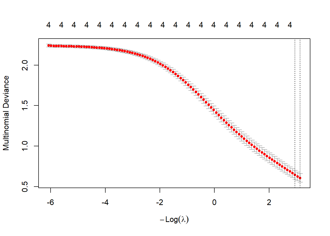
bestlam_ridge_m <- cv.ridge.m$lambda.min; bestlam_ridge_m## [1] 0.04354486# Predict on test set: class labels and probabilities
ridge.class <- predict(cv.ridge.m, s = "lambda.min",
newx = x[te_idx, ], type = "class")
ridge.prob <- predict(cv.ridge.m, s = "lambda.min",
newx = x[te_idx, ], type = "response")
table(ridge.class, y[te_idx])##
## ridge.class setosa versicolor virginica
## setosa 15 0 0
## versicolor 0 17 1
## virginica 0 0 12mean(ridge.class == y[te_idx])## [1] 0.9777778Lasso multinomial (\(\alpha=1\)) with CV:
set.seed(1)
cv.lasso.m <- cv.glmnet(x[tr_idx, ], y[tr_idx],
                family = "multinomial", alpha = 1)
plot(cv.lasso.m)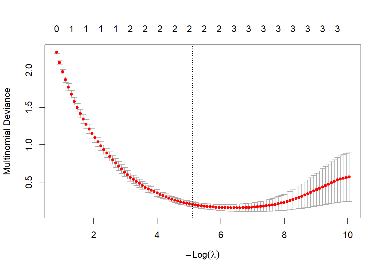
bestlam_lasso_m <- cv.lasso.m$lambda.min; bestlam_lasso_m## [1] 0.001639436lasso.class <- predict(cv.lasso.m, s = "lambda.min",
newx = x[te_idx, ], type = "class")
lasso.prob <- predict(cv.lasso.m, s = "lambda.min",
newx = x[te_idx, ], type = "response")
table(lasso.class, y[te_idx])##
## lasso.class setosa versicolor virginica
## setosa 15 0 0
## versicolor 0 17 2
## virginica 0 0 11mean(lasso.class == y[te_idx])## [1] 0.9555556Inspect sparsity (nonzero coefficients) under lasso. For multinomial, coefficients are returned per class:
lasso_coefs <- coef(cv.lasso.m$glmnet.fit, s = bestlam_lasso_m)
# lasso_coefs is a list of coefficient matrices, one per class:
names(lasso_coefs)
## [1] "setosa" "versicolor" "virginica"lasso_coefs[[1]][lasso_coefs[[1]]!= 0] # nonzeros for first class## [1] 10.8531281 2.4589078 -3.8174372 -0.0137657(Self-Study) Linear Discriminant Analysis
Now we will perform LDA on the Smarket data. In
R, we fit an LDA model using the lda()
function, which is part of the MASS library. Notice that
the syntax for the lda() function is identical to that of
lm(), and to that of glm() except for the
absence of the family option. We fit the model using only
the observations before 2005.
library(MASS)##
## Attaching package: 'MASS'## The following object is masked from 'package:ISLR2':
##
## Bostonlda.fit <- lda(Direction ~ Lag1 + Lag2, data = Smarket,
subset = train)
lda.fit## Call:
## lda(Direction ~ Lag1 + Lag2, data = Smarket, subset = train)
##
## Prior probabilities of groups:
## Down Up
## 0.5047619 0.4952381
##
## Group means:
## Lag1 Lag2
## Down 0.06139623 -0.0390000
## Up -0.19875000 -0.1391923
##
## Coefficients of linear discriminants:
## LD1
## Lag1 -0.7194761
## Lag2 -0.2670035plot(lda.fit)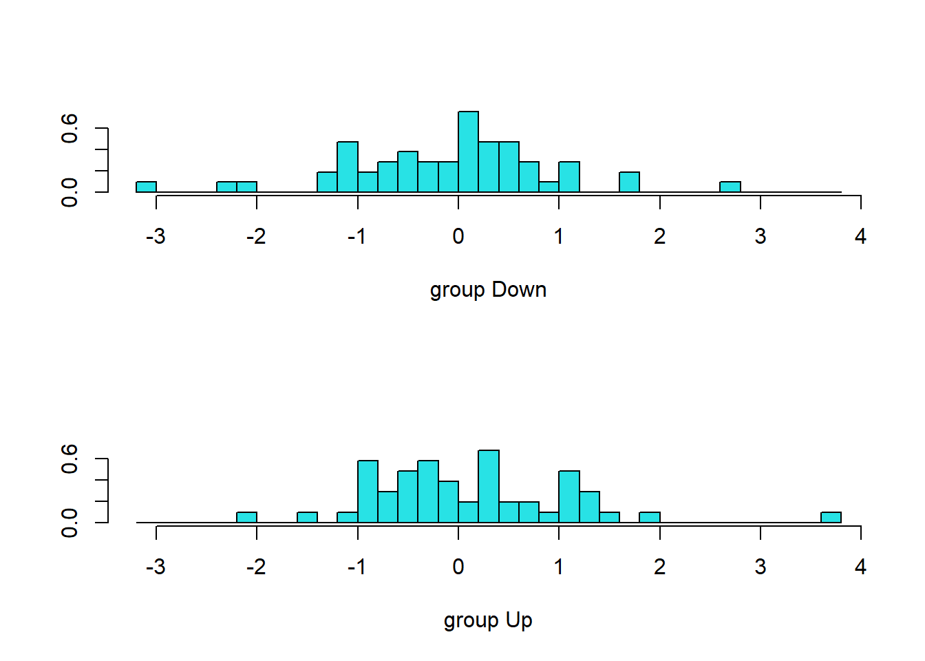
The LDA output indicates that \(\hat\pi_1=0.492\) and \(\hat\pi_2=0.508\); in other words, 49.2% of
the training observations correspond to days during which the market
went down. It also provides the group means; these are the average of
each predictor within each class, and are used by LDA as estimates of
\(\mu_k\). These suggest that there is
a tendency for the previous 2 days’ returns to be negative on days when
the market increases, and a tendency for the previous days’ returns to
be positive on days when the market declines. The coefficients of
linear discriminants output provides the linear combination of
lagone and lagtwo that are used to form the
LDA decision rule. In other words, these are the multipliers of the
elements of \(X=x\). If \(-0.642\times\)lagone\(-0.514\times\)lagtwo is large,
then the LDA classifier will predict a market increase, and if it is
small, then the LDA classifier will predict a market decline. The
plot() function produces plots of the linear
discriminants, obtained by computing \(-0.642\times\)lagone\(-0.514\times\)lagtwo for each
of the training observations. The Up and Down
observations are displayed separately.
The predict() function returns a list with three
elements. The first element, class, contains LDA’s
predictions about the movement of the market. The second element,
posterior, is a matrix whose \(k\)th column contains the posterior
probability that the corresponding observation belongs to the \(k\)th class. Finally, x
contains the linear discriminants, described earlier.
lda.pred <- predict(lda.fit, Smarket.2005)
names(lda.pred)
## [1] "class" "posterior" "x"The LDA and logistic regression predictions are almost identical.
lda.class <- lda.pred$class
table(lda.class, Direction.2005)
## Direction.2005
## lda.class Down Up
## Down 79 85
## Up 32 56mean(lda.class == Direction.2005)## [1] 0.5357143Applying a 50% threshold to the posterior probabilities allows us to
recreate the predictions contained in lda.pred$class.
sum(lda.pred$posterior[, 1] >= .5)## [1] 164sum(lda.pred$posterior[, 1] < .5)## [1] 88Notice that the posterior probability output by the model corresponds to the probability that the market will decrease:
lda.pred$posterior[1:20, 1]## 999 1000 1001 1002 1003 1004 1005 1006
## 0.5036350 0.4755390 0.4523238 0.4780595 0.5169925 0.5081858 0.5197839 0.4900903
## 1007 1008 1009 1010 1011 1012 1013 1014
## 0.5152758 0.4811627 0.5194305 0.5542381 0.4859733 0.4652461 0.4729297 0.4859448
## 1015 1016 1017 1018
## 0.5190181 0.5329639 0.5171589 0.4987963lda.class[1:20]## [1] Down Up Up Up Down Down Down Up Down Up Down Down Up Up Up
## [16] Up Down Down Down Up
## Levels: Down UpIf we wanted to use a posterior probability threshold other than 50% in order to make predictions, then we could easily do so. For instance, suppose that we wish to predict a market decrease only if we are very certain that the market will indeed decrease on that day—say, if the posterior probability is at least 90%.
sum(lda.pred$posterior[, 1] > .9)## [1] 0No days in 2005 meet that threshold! In fact, the greatest posterior probability of decrease in all of 2005 was 52.02%.
(Self-Study) Quadratic Discriminant Analysis
We will now fit a QDA model to the Smarket data. QDA is
implemented in R using the qda() function,
which is also part of the MASS library. The syntax is
identical to that of lda().
qda.fit <- qda(Direction ~ Lag1 + Lag2, data = Smarket,
    subset = train)
qda.fit
## Call:
## qda(Direction ~ Lag1 + Lag2, data = Smarket, subset = train)
##
## Prior probabilities of groups:
## Down Up
## 0.5047619 0.4952381
##
## Group means:
## Lag1 Lag2
## Down 0.06139623 -0.0390000
## Up -0.19875000 -0.1391923The output contains the group means. But it does not contain the
coefficients of the linear discriminants, because the QDA classifier
involves a quadratic, rather than a linear, function of the predictors.
The predict() function works in exactly the same fashion as
for LDA.
qda.class <- predict(qda.fit, Smarket.2005)$class
table(qda.class, Direction.2005)
## Direction.2005
## qda.class Down Up
## Down 13 17
## Up 98 124mean(qda.class == Direction.2005)## [1] 0.5436508Interestingly, the QDA predictions are accurate almost 60% of the time, even though the 2005 data was not used to fit the model. This level of accuracy is quite impressive for stock market data, which is known to be quite hard to model accurately. This suggests that the quadratic form assumed by QDA may capture the true relationship more accurately than the linear forms assumed by LDA and logistic regression. However, we recommend evaluating this method’s performance on a larger test set before betting that this approach will consistently beat the market!
(Self-Study) Naive Bayes
Next, we fit a naive Bayes model to the Smarket data.
Naive Bayes is implemented in R using the
naiveBayes() function, which is part of the
e1071 library. The syntax is identical to that of
lda() and qda(). By default, this
implementation of the naive Bayes classifier models each quantitative
feature using a Gaussian distribution. However, a kernel density method
can also be used to estimate the distributions.
library(e1071)
nb.fit <- naiveBayes(Direction ~ Lag1 + Lag2, data = Smarket,
    subset = train)
nb.fit
##
## Naive Bayes Classifier for Discrete Predictors
##
## Call:
## naiveBayes.default(x = X, y = Y, laplace = laplace)
##
## A-priori probabilities:
## Y
## Down Up
## 0.5047619 0.4952381
##
## Conditional probabilities:
## Lag1
## Y [,1] [,2]
## Down 0.06139623 1.371229
## Up -0.19875000 1.190518
##
## Lag2
## Y [,1] [,2]
## Down -0.0390000 1.302211
## Up -0.1391923 1.113083The output contains the estimated mean and standard deviation for
each variable in each class. For example, the mean for
lagone is 0.0428 for Direction=Down, and the
standard deviation is 1.23. We can easily verify this:
mean(Lag1[train][Direction[train] == "Down"])## [1] 0.06139623sd(Lag1[train][Direction[train] == "Down"])## [1] 1.371229The predict() function is straightforward.
nb.class <- predict(nb.fit, Smarket.2005)
table(nb.class, Direction.2005)
## Direction.2005
## nb.class Down Up
## Down 15 15
## Up 96 126mean(nb.class == Direction.2005)## [1] 0.5595238Naive Bayes performs very well on this data, with accurate predictions over 59% of the time. This is slightly worse than QDA, but much better than LDA.
The predict() function can also generate estimates of
the probability that each observation belongs to a particular class.
nb.preds <- predict(nb.fit, Smarket.2005, type = "raw")
nb.preds[1:5, ]
## Down Up
## [1,] 0.4305071 0.5694929
## [2,] 0.4128903 0.5871097
## [3,] 0.4150242 0.5849758
## [4,] 0.4337853 0.5662147
## [5,] 0.4487743 0.5512257