Supervised Learning IV - Decision Trees and Ensemble Methods
Patrick PUN Chi Seng (NTU Sg)
References
Chapters 8.3 [ISLR2] An Introduction to Statistical Learning - with Applications in R (2nd Edition). Free access to download the book: https://www.statlearning.com/
To see the help file of a function funcname, type
?funcname.
Fitting Classification Trees
The tree library is used to construct classification and
regression trees.
library(tree)We first use classification trees to analyze the
Carseats data set. In these data, Sales is a
continuous variable, and so we begin by recoding it as a binary
variable. We use the ifelse() function to create a
variable, called High, which takes on a value of
Yes if the Sales variable exceeds 8, and takes
on a value of No otherwise.
library(ISLR2)
attach(Carseats)
High <- factor(ifelse(Sales <= 8, "No", "Yes"))
Finally, we use the data.frame() function to merge
High with the rest of the Carseats data.
Carseats <- data.frame(Carseats, High)We now use the tree() function to fit a classification
tree in order to predict High using all variables but
Sales. The syntax of the tree() function is
quite similar to that of the lm() function.
tree.carseats <- tree(High ~ . - Sales, Carseats)The summary() function lists the variables that are used
as internal nodes in the tree, the number of terminal nodes, and the
(training) error rate.
summary(tree.carseats)##
## Classification tree:
## tree(formula = High ~ . - Sales, data = Carseats)
## Variables actually used in tree construction:
## [1] "ShelveLoc" "Price" "Income" "CompPrice" "Population"
## [6] "Advertising" "Age" "US"
## Number of terminal nodes: 27
## Residual mean deviance: 0.4575 = 170.7 / 373
## Misclassification error rate: 0.09 = 36 / 400We see that the training error rate is 9%. For classification trees,
the deviance reported in the output of summary() is given
by \[
-2 \sum_m \sum_k n_{mk} \log \hat{p}_{mk},
\] where \(n_{mk}\) is the
number of observations in the \(m\)th
terminal node that belong to the \(k\)th class. This is closely related to the
entropy, defined in (8.7). A small deviance indicates a tree that
provides a good fit to the (training) data. The residual mean
deviance reported is simply the deviance divided by \(n-|{T}_0|\), which in this case is
400-27=373.
One of the most attractive properties of trees is that they can be
graphically displayed. We use the plot() function to
display the tree structure, and the text() function to
display the node labels. The argument pretty = 0 instructs
R to include the category names for any qualitative
predictors, rather than simply displaying a letter for each
category.
plot(tree.carseats)
text(tree.carseats, pretty = 0)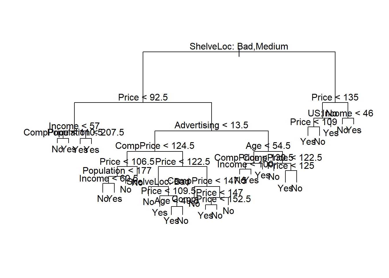
The most important indicator of Sales appears to be
shelving location, since the first branch differentiates
Good locations from Bad and
Medium locations.
If we just type the name of the tree object, R prints
output corresponding to each branch of the tree. R displays
the split criterion (e.g. Price < 92.5), the number of
observations in that branch, the deviance, the overall prediction for
the branch (Yes or No), and the fraction of
observations in that branch that take on values of Yes and
No. Branches that lead to terminal nodes are indicated
using asterisks.
tree.carseats## node), split, n, deviance, yval, (yprob)
## * denotes terminal node
##
## 1) root 400 541.500 No ( 0.59000 0.41000 )
## 2) ShelveLoc: Bad,Medium 315 390.600 No ( 0.68889 0.31111 )
## 4) Price < 92.5 46 56.530 Yes ( 0.30435 0.69565 )
## 8) Income < 57 10 12.220 No ( 0.70000 0.30000 )
## 16) CompPrice < 110.5 5 0.000 No ( 1.00000 0.00000 ) *
## 17) CompPrice > 110.5 5 6.730 Yes ( 0.40000 0.60000 ) *
## 9) Income > 57 36 35.470 Yes ( 0.19444 0.80556 )
## 18) Population < 207.5 16 21.170 Yes ( 0.37500 0.62500 ) *
## 19) Population > 207.5 20 7.941 Yes ( 0.05000 0.95000 ) *
## 5) Price > 92.5 269 299.800 No ( 0.75465 0.24535 )
## 10) Advertising < 13.5 224 213.200 No ( 0.81696 0.18304 )
## 20) CompPrice < 124.5 96 44.890 No ( 0.93750 0.06250 )
## 40) Price < 106.5 38 33.150 No ( 0.84211 0.15789 )
## 80) Population < 177 12 16.300 No ( 0.58333 0.41667 )
## 160) Income < 60.5 6 0.000 No ( 1.00000 0.00000 ) *
## 161) Income > 60.5 6 5.407 Yes ( 0.16667 0.83333 ) *
## 81) Population > 177 26 8.477 No ( 0.96154 0.03846 ) *
## 41) Price > 106.5 58 0.000 No ( 1.00000 0.00000 ) *
## 21) CompPrice > 124.5 128 150.200 No ( 0.72656 0.27344 )
## 42) Price < 122.5 51 70.680 Yes ( 0.49020 0.50980 )
## 84) ShelveLoc: Bad 11 6.702 No ( 0.90909 0.09091 ) *
## 85) ShelveLoc: Medium 40 52.930 Yes ( 0.37500 0.62500 )
## 170) Price < 109.5 16 7.481 Yes ( 0.06250 0.93750 ) *
## 171) Price > 109.5 24 32.600 No ( 0.58333 0.41667 )
## 342) Age < 49.5 13 16.050 Yes ( 0.30769 0.69231 ) *
## 343) Age > 49.5 11 6.702 No ( 0.90909 0.09091 ) *
## 43) Price > 122.5 77 55.540 No ( 0.88312 0.11688 )
## 86) CompPrice < 147.5 58 17.400 No ( 0.96552 0.03448 ) *
## 87) CompPrice > 147.5 19 25.010 No ( 0.63158 0.36842 )
## 174) Price < 147 12 16.300 Yes ( 0.41667 0.58333 )
## 348) CompPrice < 152.5 7 5.742 Yes ( 0.14286 0.85714 ) *
## 349) CompPrice > 152.5 5 5.004 No ( 0.80000 0.20000 ) *
## 175) Price > 147 7 0.000 No ( 1.00000 0.00000 ) *
## 11) Advertising > 13.5 45 61.830 Yes ( 0.44444 0.55556 )
## 22) Age < 54.5 25 25.020 Yes ( 0.20000 0.80000 )
## 44) CompPrice < 130.5 14 18.250 Yes ( 0.35714 0.64286 )
## 88) Income < 100 9 12.370 No ( 0.55556 0.44444 ) *
## 89) Income > 100 5 0.000 Yes ( 0.00000 1.00000 ) *
## 45) CompPrice > 130.5 11 0.000 Yes ( 0.00000 1.00000 ) *
## 23) Age > 54.5 20 22.490 No ( 0.75000 0.25000 )
## 46) CompPrice < 122.5 10 0.000 No ( 1.00000 0.00000 ) *
## 47) CompPrice > 122.5 10 13.860 No ( 0.50000 0.50000 )
## 94) Price < 125 5 0.000 Yes ( 0.00000 1.00000 ) *
## 95) Price > 125 5 0.000 No ( 1.00000 0.00000 ) *
## 3) ShelveLoc: Good 85 90.330 Yes ( 0.22353 0.77647 )
## 6) Price < 135 68 49.260 Yes ( 0.11765 0.88235 )
## 12) US: No 17 22.070 Yes ( 0.35294 0.64706 )
## 24) Price < 109 8 0.000 Yes ( 0.00000 1.00000 ) *
## 25) Price > 109 9 11.460 No ( 0.66667 0.33333 ) *
## 13) US: Yes 51 16.880 Yes ( 0.03922 0.96078 ) *
## 7) Price > 135 17 22.070 No ( 0.64706 0.35294 )
## 14) Income < 46 6 0.000 No ( 1.00000 0.00000 ) *
## 15) Income > 46 11 15.160 Yes ( 0.45455 0.54545 ) *In order to properly evaluate the performance of a classification
tree on these data, we must estimate the test error rather than simply
computing the training error. We split the observations into a training
set and a test set, build the tree using the training set, and evaluate
its performance on the test data. The predict() function
can be used for this purpose. In the case of a classification tree, the
argument type = "class" instructs R to return
the actual class prediction. This approach leads to correct predictions
for around 77% of the locations in the test data set.
set.seed(2)
train <- sample(1:nrow(Carseats), 200)
Carseats.test <- Carseats[-train, ]
High.test <- High[-train]
tree.carseats <- tree(High ~ . - Sales, Carseats,
    subset = train)
tree.pred <- predict(tree.carseats, Carseats.test,
    type = "class")
table(tree.pred, High.test)
## High.test
## tree.pred No Yes
## No 104 33
## Yes 13 50(104 + 50) / 200## [1] 0.77(If you re-run the predict() function then you might get
slightly different results, due to “ties”: for instance, this can happen
when the training observations corresponding to a terminal node are
evenly split between Yes and No response
values.)
Next, we consider whether pruning the tree might lead to improved
results. The function cv.tree() performs cross-validation
in order to determine the optimal level of tree complexity; cost
complexity pruning is used in order to select a sequence of trees for
consideration. We use the argument FUN = prune.misclass in
order to indicate that we want the classification error rate to guide
the cross-validation and pruning process, rather than the default for
the cv.tree() function, which is deviance. The
cv.tree() function reports the number of terminal nodes of
each tree considered (size) as well as the corresponding
error rate and the value of the cost-complexity parameter used
(k, which corresponds to \(\alpha\) in (8.4)).
set.seed(7)
cv.carseats <- cv.tree(tree.carseats, FUN = prune.misclass)
names(cv.carseats)
## [1] "size" "dev" "k" "method"cv.carseats## $size
## [1] 21 19 14 9 8 5 3 2 1
##
## $dev
## [1] 75 75 75 74 82 83 83 85 82
##
## $k
## [1] -Inf 0.0 1.0 1.4 2.0 3.0 4.0 9.0 18.0
##
## $method
## [1] "misclass"
##
## attr(,"class")
## [1] "prune" "tree.sequence"Despite its name, dev corresponds to the number of
cross-validation errors. The tree with 9 terminal nodes results in only
74 cross-validation errors. We plot the error rate as a function of both
size and k.
par(mfrow = c(1, 2))
plot(cv.carseats$size, cv.carseats$dev, type = "b")
plot(cv.carseats$k, cv.carseats$dev, type = "b")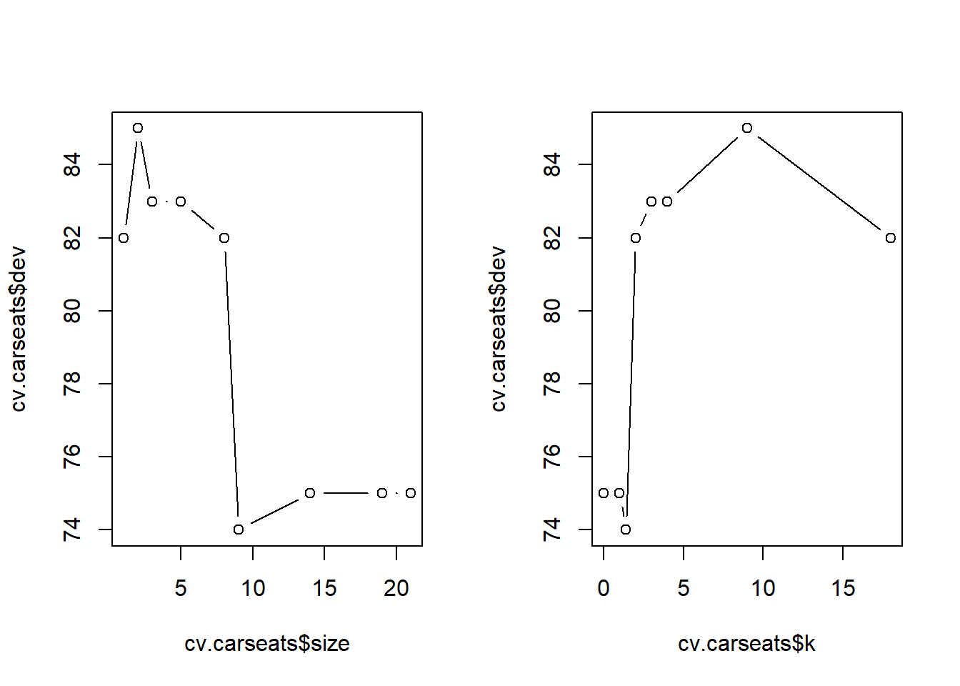
We now apply the prune.misclass() function in order to
prune the tree to obtain the nine-node tree.
prune.carseats <- prune.misclass(tree.carseats, best = 9)
plot(prune.carseats)
text(prune.carseats, pretty = 0)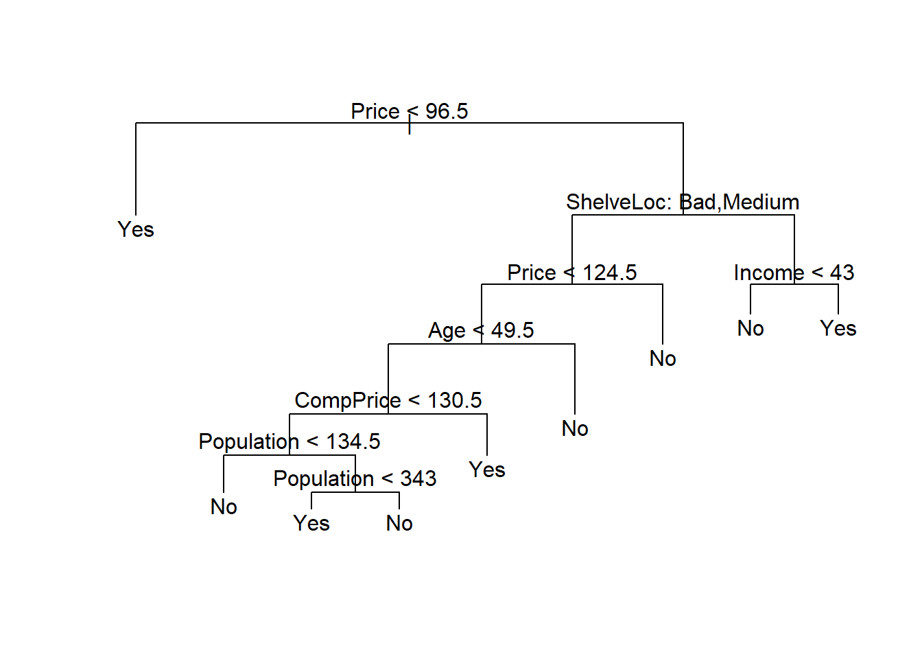
How well does this pruned tree perform on the test data set? Once
again, we apply the predict() function.
tree.pred <- predict(prune.carseats, Carseats.test,
    type = "class")
table(tree.pred, High.test)
## High.test
## tree.pred No Yes
## No 97 25
## Yes 20 58(97 + 58) / 200## [1] 0.775Now 77.5% of the test observations are correctly classified, so not only has the pruning process produced a more interpretable tree, but it has also slightly improved the classification accuracy.
If we increase the value of best, we obtain a larger
pruned tree with lower classification accuracy:
prune.carseats <- prune.misclass(tree.carseats, best = 14)
plot(prune.carseats)
text(prune.carseats, pretty = 0)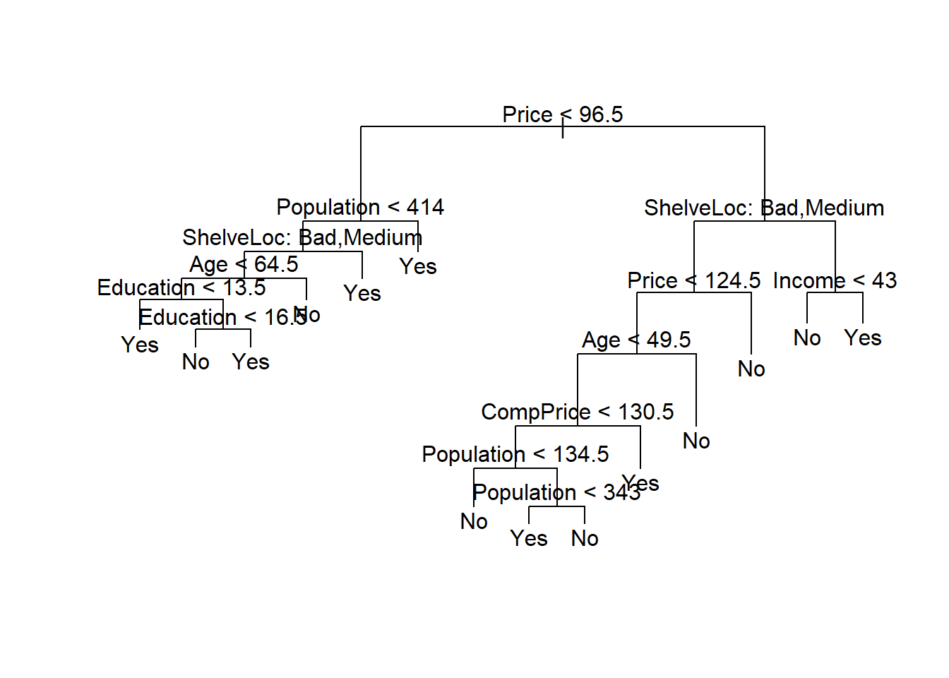
tree.pred <- predict(prune.carseats, Carseats.test,
    type = "class")
table(tree.pred, High.test)
## High.test
## tree.pred No Yes
## No 102 31
## Yes 15 52(102 + 52) / 200## [1] 0.77Fitting Regression Trees
Here we fit a regression tree to the Boston data set.
First, we create a training set, and fit the tree to the training
data.
set.seed(1)
train <- sample(1:nrow(Boston), nrow(Boston) / 2)
tree.boston <- tree(medv ~ ., Boston, subset = train)
summary(tree.boston)
##
## Regression tree:
## tree(formula = medv ~ ., data = Boston, subset = train)
## Variables actually used in tree construction:
## [1] "rm" "lstat" "crim" "age"
## Number of terminal nodes: 7
## Residual mean deviance: 10.38 = 2555 / 246
## Distribution of residuals:
## Min. 1st Qu. Median Mean 3rd Qu. Max.
## -10.1800 -1.7770 -0.1775 0.0000 1.9230 16.5800Notice that the output of summary() indicates that only
four of the variables have been used in constructing the tree. In the
context of a regression tree, the deviance is simply the sum of squared
errors for the tree. We now plot the tree.
plot(tree.boston)
text(tree.boston, pretty = 0)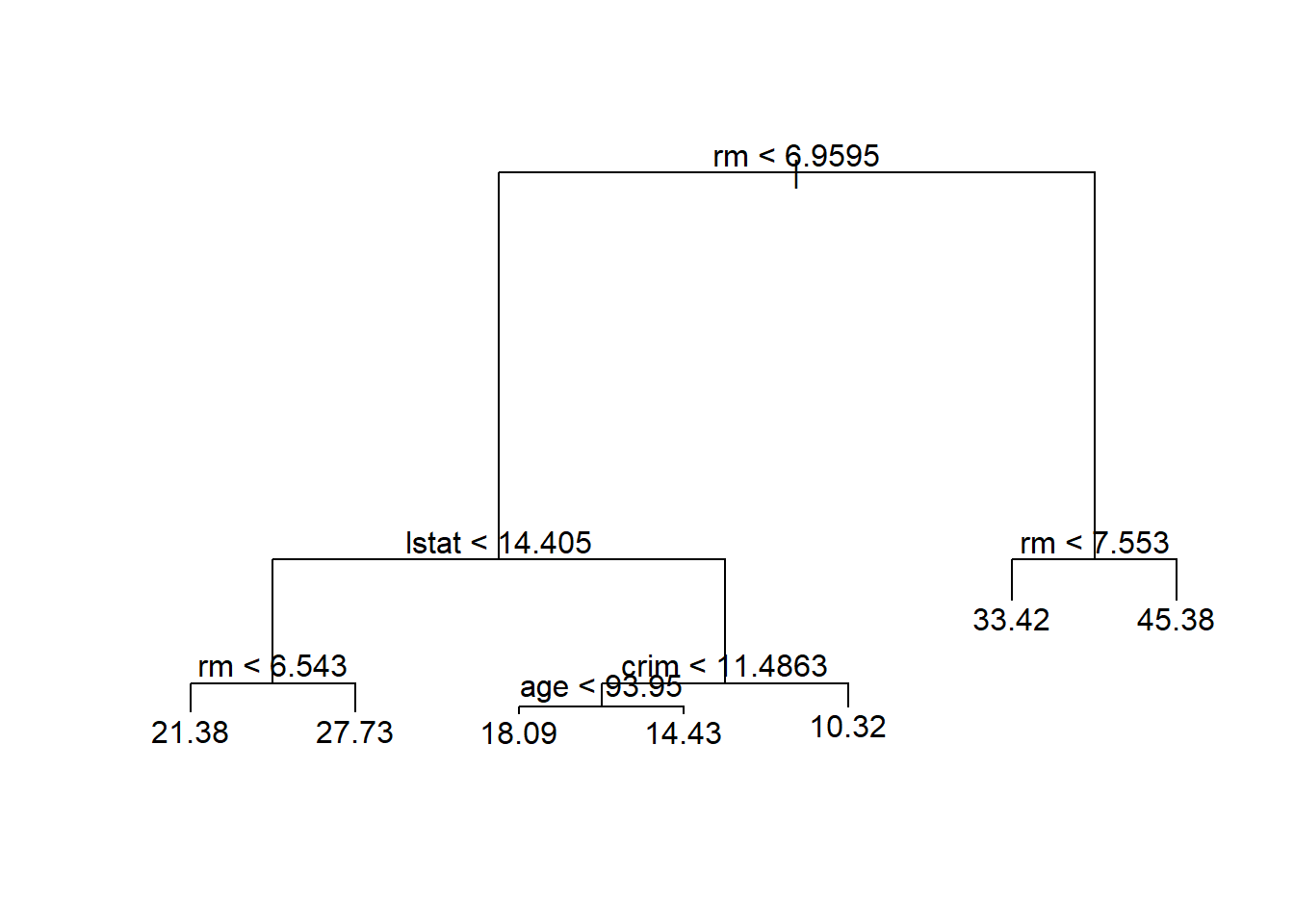
The variable lstat measures the percentage of
individuals with {lower socioeconomic status}, while the variable
rm corresponds to the average number of rooms. The tree
indicates that larger values of rm, or lower values of
lstat, correspond to more expensive houses. For example,
the tree predicts a median house price of 45,400 for homes in census
tracts in which rm >= 7.553.
It is worth noting that we could have fit a much bigger tree, by
passing
control = tree.control(nobs = length(train), mindev = 0)
into the tree() function.
Now we use the cv.tree() function to see whether pruning
the tree will improve performance.
cv.boston <- cv.tree(tree.boston)
plot(cv.boston$size, cv.boston$dev, type = "b")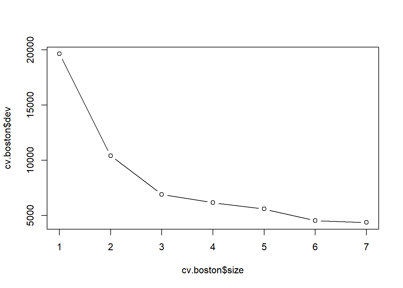
In this case, the most complex tree under consideration is selected
by cross-validation. However, if we wish to prune the tree, we could do
so as follows, using the prune.tree() function:
prune.boston <- prune.tree(tree.boston, best = 5)
plot(prune.boston)
text(prune.boston, pretty = 0)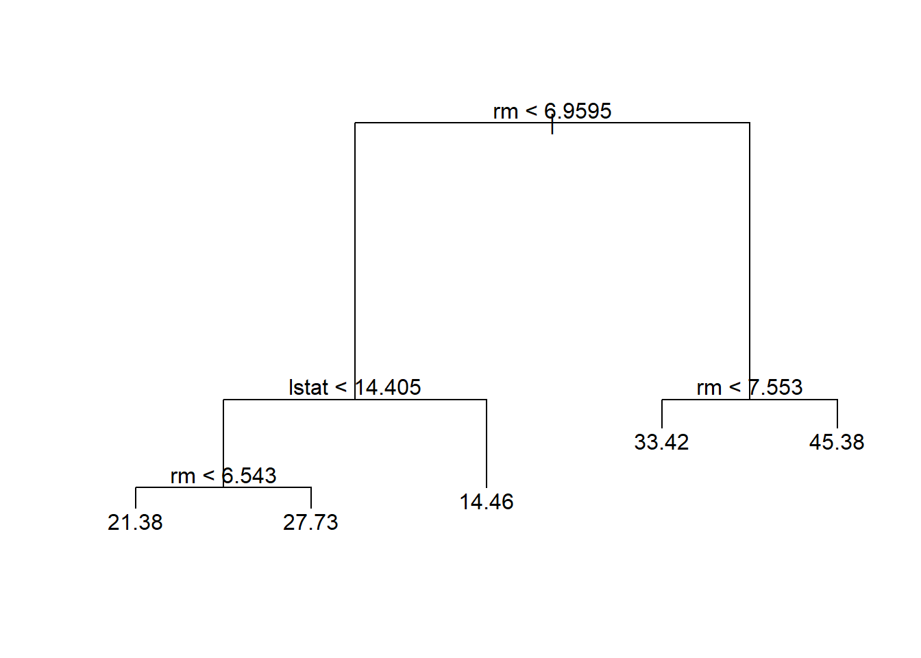
In keeping with the cross-validation results, we use the unpruned tree to make predictions on the test set.
yhat <- predict(tree.boston, newdata = Boston[-train, ])
boston.test <- Boston[-train, "medv"]
plot(yhat, boston.test)
abline(0, 1)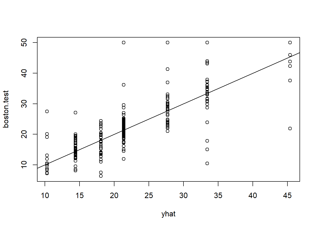
mean((yhat - boston.test)^2)## [1] 35.28688In other words, the test set MSE associated with the regression tree is 35.29. The square root of the MSE is therefore around 5.941, indicating that this model leads to test predictions that are (on average) within approximately 5,941 of the true median home value for the census tract.
Bagging and Random Forests
Here we apply bagging and random forests to the Boston
data, using the randomForest package in R. The
exact results obtained in this section may depend on the version of
R and the version of the randomForest package
installed on your computer. Recall that bagging is simply a special case
of a random forest with \(m=p\).
Therefore, the randomForest() function can be used to
perform both random forests and bagging.
We perform bagging as follows:
library(randomForest)## randomForest 4.7-1.2## Type rfNews() to see new features/changes/bug fixes.set.seed(1)
bag.boston <- randomForest(medv ~ ., data = Boston, subset = train, mtry = 12, importance = TRUE)
bag.boston##
## Call:
## randomForest(formula = medv ~ ., data = Boston, mtry = 12, importance = TRUE, subset = train)
## Type of random forest: regression
## Number of trees: 500
## No. of variables tried at each split: 12
##
## Mean of squared residuals: 11.40162
## % Var explained: 85.17The argument mtry = 12 indicates that all 12 predictors
should be considered for each split of the tree—in other words, that
bagging should be done. How well does this bagged model perform on the
test set?
yhat.bag <- predict(bag.boston, newdata = Boston[-train, ])
plot(yhat.bag, boston.test)
abline(0, 1)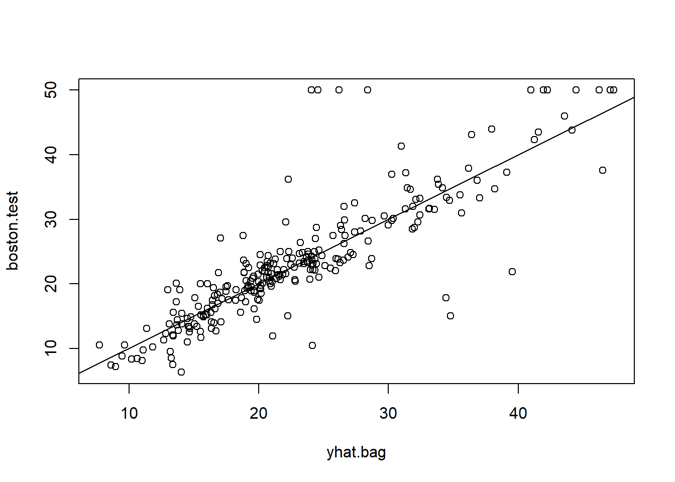
mean((yhat.bag - boston.test)^2)## [1] 23.41916The test set MSE associated with the bagged regression tree is 23.42,
about two-thirds of that obtained using an optimally-pruned single tree.
We could change the number of trees grown by randomForest()
using the ntree argument:
bag.boston <- randomForest(medv ~ ., data = Boston,
    subset = train, mtry = 12, ntree = 25)
yhat.bag <- predict(bag.boston, newdata = Boston[-train, ])
mean((yhat.bag - boston.test)^2)
## [1] 25.75055Growing a random forest proceeds in exactly the same way, except that
we use a smaller value of the mtry argument. By default,
randomForest() uses \(p/3\) variables when building a random
forest of regression trees, and \(\sqrt{p}\) variables when building a random
forest of classification trees. Here we use mtry = 6.
set.seed(1)
rf.boston <- randomForest(medv ~ ., data = Boston,
    subset = train, mtry = 6, importance = TRUE)
yhat.rf <- predict(rf.boston, newdata = Boston[-train, ])
mean((yhat.rf - boston.test)^2)
## [1] 20.06644The test set MSE is 20.07; this indicates that random forests yielded an improvement over bagging in this case.
Using the importance() function, we can view the
importance of each variable.
importance(rf.boston)## %IncMSE IncNodePurity
## crim 19.435587 1070.42307
## zn 3.091630 82.19257
## indus 6.140529 590.09536
## chas 1.370310 36.70356
## nox 13.263466 859.97091
## rm 35.094741 8270.33906
## age 15.144821 634.31220
## dis 9.163776 684.87953
## rad 4.793720 83.18719
## tax 4.410714 292.20949
## ptratio 8.612780 902.20190
## lstat 28.725343 5813.04833Two measures of variable importance are reported. The first is based
upon the mean decrease of accuracy in predictions on the out of bag
samples when a given variable is permuted. The second is a measure of
the total decrease in node impurity that results from splits over that
variable, averaged over all trees (this was plotted in Figure 8.9). In
the case of regression trees, the node impurity is measured by the
training RSS, and for classification trees by the deviance. Plots of
these importance measures can be produced using the
varImpPlot() function.
varImpPlot(rf.boston)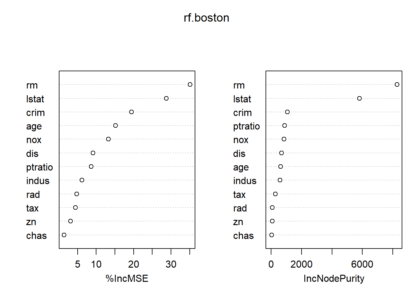
The results indicate that across all of the trees considered in the
random forest, the wealth of the community (lstat) and the
house size (rm) are by far the two most important
variables.
Boosting
Here we use the gbm package, and within it the
gbm() function, to fit boosted regression trees to the
Boston data set. We run gbm() with the option
distribution = "gaussian" since this is a regression
problem; if it were a binary classification problem, we would use
distribution = "bernoulli". The argument
n.trees = 5000 indicates that we want 5000 trees, and the
option interaction.depth = 4 limits the depth of each
tree.
library(gbm)## Loaded gbm 2.2.2## This version of gbm is no longer under development. Consider transitioning to gbm3, https://github.com/gbm-developers/gbm3set.seed(1)
boost.boston <- gbm(medv ~ ., data = Boston[train, ],
distribution = "gaussian", n.trees = 5000,
interaction.depth = 4)The summary() function produces a relative influence
plot and also outputs the relative influence statistics.
summary(boost.boston)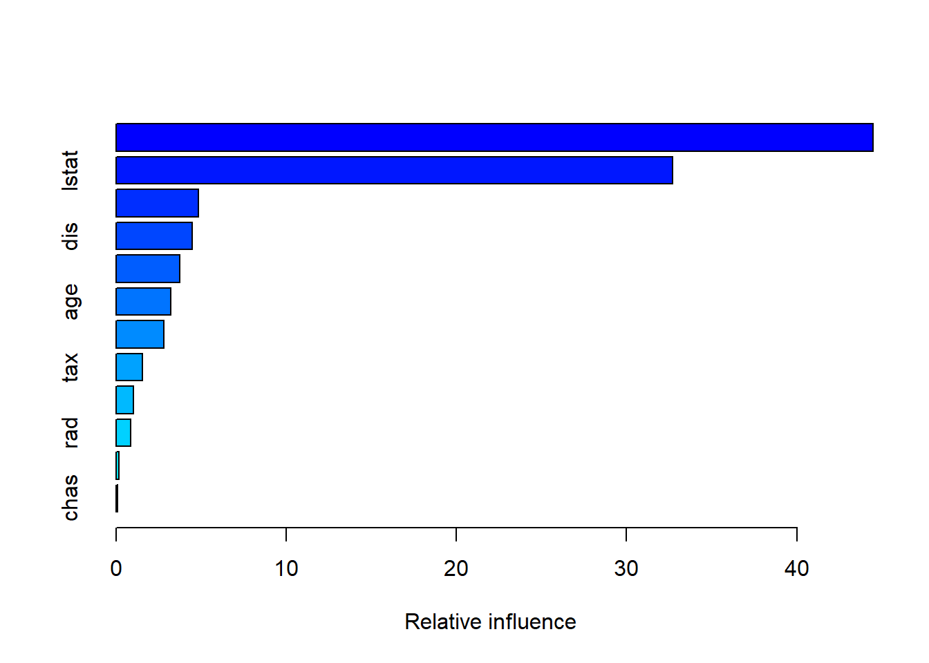
We see that lstat and rm are by far the
most important variables. We can also produce partial dependence
plots for these two variables. These plots illustrate the marginal
effect of the selected variables on the response after
integrating out the other variables. In this case, as we might
expect, median house prices are increasing with rm and
decreasing with lstat.
plot(boost.boston, i = "rm")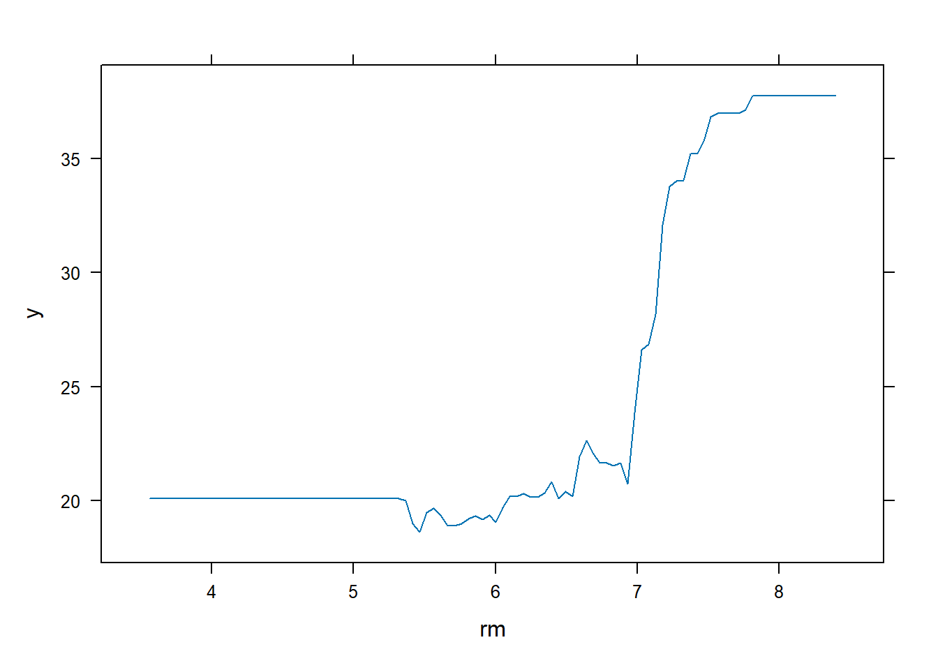
plot(boost.boston, i = "lstat")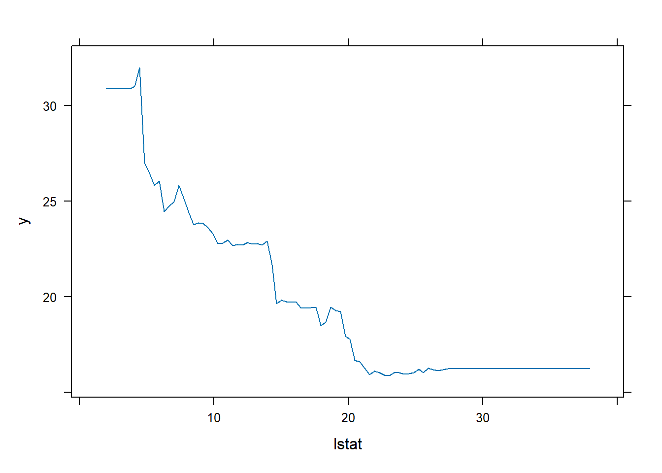
We now use the boosted model to predict medv on the test
set:
yhat.boost <- predict(boost.boston,
    newdata = Boston[-train, ], n.trees = 5000)
mean((yhat.boost - boston.test)^2)
## [1] 18.39057The test MSE obtained is 18.39: this is superior to the test MSE of random forests and bagging. If we want to, we can perform boosting with a different value of the shrinkage parameter \(\lambda\) in (8.10). The default value is 0.001, but this is easily modified. Here we take \(\lambda=0.2\).
boost.boston <- gbm(medv ~ ., data = Boston[train, ],
    distribution = "gaussian", n.trees = 5000,
    interaction.depth = 4, shrinkage = 0.2, verbose = F)
yhat.boost <- predict(boost.boston,
    newdata = Boston[-train, ], n.trees = 5000)
mean((yhat.boost - boston.test)^2)
## [1] 16.54778In this case, using \(\lambda=0.2\) leads to a lower test MSE than \(\lambda=0.001\).
Adaptive Boosting (AdaBoost)
AdaBoost (Adaptive Boosting) is an ensemble method that builds a strong classifier from a set of weak classifiers, typically shallow trees. Misclassified observations are given more weight in subsequent rounds, forcing the algorithm to focus on harder cases.
We use the JOUSBoost package. Here, the response
variable is coded as +1 (Yes) and -1 (No).
# install.packages("JOUSBoost")
library(JOUSBoost)
## JOUSBoost 2.1.0library(MASS)##
## Attaching package: 'MASS'## The following object is masked from 'package:ISLR2':
##
## Bostondata(Boston)
Boston.cls <- Boston
Boston.cls$cmed <- "No"
Boston.cls$cmed[Boston.cls$crim > median(Boston.cls[train,]$crim)] <- "Yes"
Boston.cls$cmed <- factor(Boston.cls$cmed)
Boston.cls <- Boston.cls[,-1] # drop the crim variable
# Encode response as +1/-1
y <- rep(1, nrow(Boston.cls[train, ]))
y[Boston.cls[train, ]$cmed == "No"] <- -1
X <- as.matrix(Boston.cls[train, -ncol(Boston.cls)])
# Train AdaBoost classifier with depth-5 trees
ada.cls <- adaboost(X, y, tree_depth = 5, n_rounds = 100)
ada.cls## AdaBoost: tree_depth = 5 rounds = 100
##
##
## In-sample confusion matrix:
## yhat
## y -1 1
## -1 127 0
## 1 0 126# Predict on test set
ada.pred <- predict(ada.cls, Boston.cls[-train, ])
cmed.true <- Boston.cls$cmed[-train]
ada.cm <- table(ada.pred, cmed.true); ada.cm## cmed.true
## ada.pred No Yes
## -1 122 17
## 1 4 110# Misclassification rate
1 - sum(diag(ada.cm)) / sum(ada.cm)## [1] 0.08300395The confusion matrix shows how well AdaBoost separates the two classes, and the misclassification rate provides the test error estimate.
Extreme Gradient Boosting (XGBoost)
XGBoost is a more scalable and efficient boosting implementation that
supports both regression and classification. It uses second-order
gradient information for optimization, regularization to avoid
overfitting, and allows for fine-grained tuning of tree depth, learning
rate (eta), and number of boosting rounds.
We use the xgboost package and recode the response as 1
(Yes) and 0 (No).
# install.packages("xgboost")
library(xgboost)

# Prepare training data
X.train <- as.matrix(Boston.cls[train, -ncol(Boston.cls)])
y.train <- rep(1, nrow(Boston.cls[train, ]))
y.train[Boston.cls[train, ]$cmed == "No"] <- 0

# Train XGBoost classifier
xgb.cls <- xgboost(
  data = X.train, label = y.train,
  max_depth = 5, eta = 0.01,
  nrounds = 100, verbose = FALSE
)
xgb.cls
## ##### xgb.Booster
## raw: 159.4 Kb
## call:
## xgb.train(params = params, data = dtrain, nrounds = nrounds,
## watchlist = watchlist, verbose = verbose, print_every_n = print_every_n,
## early_stopping_rounds = early_stopping_rounds, maximize = maximize,
## save_period = save_period, save_name = save_name, xgb_model = xgb_model,
## callbacks = callbacks, max_depth = 5, eta = 0.01)
## params (as set within xgb.train):
## max_depth = "5", eta = "0.01", validate_parameters = "1"
## xgb.attributes:
## niter
## callbacks:
## cb.evaluation.log()
## # of features: 13
## niter: 100
## nfeatures : 13
## evaluation_log:
## iter train_rmse
## <num> <num>
## 1 0.4956291
## 2 0.4913044
## --- ---
## 99 0.2282899
## 100 0.2267798# Predict on test set
X.test <- as.matrix(Boston.cls[-train, -ncol(Boston.cls)])
xgb.pred.prob <- predict(xgb.cls, X.test)
xgb.pred <- as.numeric(xgb.pred.prob > 0.5)
# Confusion matrix and error rate
xgb.cm <- table(xgb.pred, cmed.true); xgb.cm## cmed.true
## xgb.pred No Yes
## 0 125 19
## 1 1 1081 - sum(diag(xgb.cm)) / sum(xgb.cm)## [1] 0.07905138The test error rate can be compared with that of AdaBoost and
classical gradient boosting (gbm). Often, XGBoost provides
superior performance, especially when hyperparameters (learning rate,
depth, number of rounds) are tuned.