Supervised Learning V - Support Vector Machines
Patrick PUN Chi Seng (NTU Sg)
References
Chapter 9.6 [ISLR2] An Introduction to Statistical Learning - with Applications in R (2nd Edition). Free access to download the book: https://www.statlearning.com/
To see the help file of a function funcname, type
?funcname.
We use the e1071 library in R to
demonstrate the support vector classifier and the SVM. Another option is
the LiblineaR library, which is useful for very large
linear problems.
Support Vector Classifier
The e1071 library contains implementations for a number
of statistical learning methods. In particular, the svm()
function can be used to fit a support vector classifier when the
argument kernel = "linear" is used. This function uses a
slightly different formulation from lecture slides for the support
vector classifier.A cost argument allows us to specify the
cost of a violation to the margin. When the cost argument
is small, then the margins will be wide and many support vectors will be
on the margin or will violate the margin. When the cost
argument is large, then the margins will be narrow and there will be few
support vectors on the margin or violating the margin.
We now use the svm() function to fit the support vector
classifier for a given value of the cost parameter. Here we
demonstrate the use of this function on a two-dimensional example so
that we can plot the resulting decision boundary. We begin by generating
the observations, which belong to two classes, and checking whether the
classes are linearly separable.
set.seed(1)
x <- matrix(rnorm(20 * 2), ncol = 2)
y <- c(rep(-1, 10), rep(1, 10))
x[y == 1, ] <- x[y == 1, ] + 1
plot(x, col = (3 - y))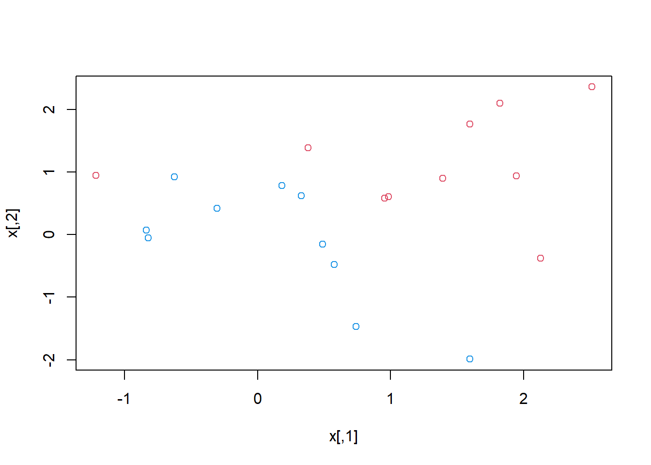
They are not. Next, we fit the support vector classifier. Note that
in order for the svm() function to perform classification
(as opposed to SVM-based regression), we must encode the response as a
factor variable. We now create a data frame with the response coded as a
factor.
dat <- data.frame(x = x, y = as.factor(y))
library(e1071)
svmfit <- svm(y ~ ., data = dat, kernel = "linear",
    cost = 10, scale = FALSE)
The argument scale = FALSE tells the svm()
function not to scale each feature to have mean zero or standard
deviation one; depending on the application, one might prefer to use
scale = TRUE.
We can now plot the support vector classifier obtained:
plot(svmfit, dat)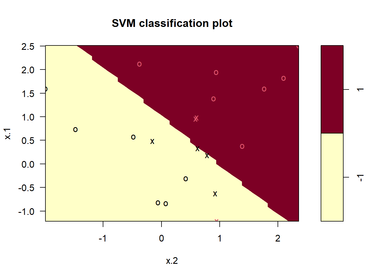
Note that the two arguments to the SVM plot() function
are the output of the call to svm(), as well as the data
used in the call to svm(). The region of feature space that
will be assigned to the -1 class is shown in light yellow, and the
region that will be assigned to the +1 class is shown in red. The
decision boundary between the two classes is linear (because we used the
argument kernel = "linear"), though due to the way in which
the plotting function is implemented in this library the decision
boundary looks somewhat jagged in the plot. (Note that here the second
feature is plotted on the \(x\)-axis
and the first feature is plotted on the \(y\)-axis, in contrast to the behavior of
the usual plot() function in R.) The support
vectors are plotted as crosses and the remaining observations are
plotted as circles; we see here that there are seven support vectors. We
can determine their identities as follows:
svmfit$index## [1] 1 2 5 7 14 16 17We can obtain some basic information about the support vector
classifier fit using the summary() command:
summary(svmfit)##
## Call:
## svm(formula = y ~ ., data = dat, kernel = "linear", cost = 10, scale = FALSE)
##
##
## Parameters:
## SVM-Type: C-classification
## SVM-Kernel: linear
## cost: 10
##
## Number of Support Vectors: 7
##
## ( 4 3 )
##
##
## Number of Classes: 2
##
## Levels:
## -1 1This tells us, for instance, that a linear kernel was used with
cost = 10, and that there were seven support vectors, four
in one class and three in the other.
What if we instead used a smaller value of the cost parameter?
svmfit <- svm(y ~ ., data = dat, kernel = "linear",
    cost = 0.1, scale = FALSE)
plot(svmfit, dat)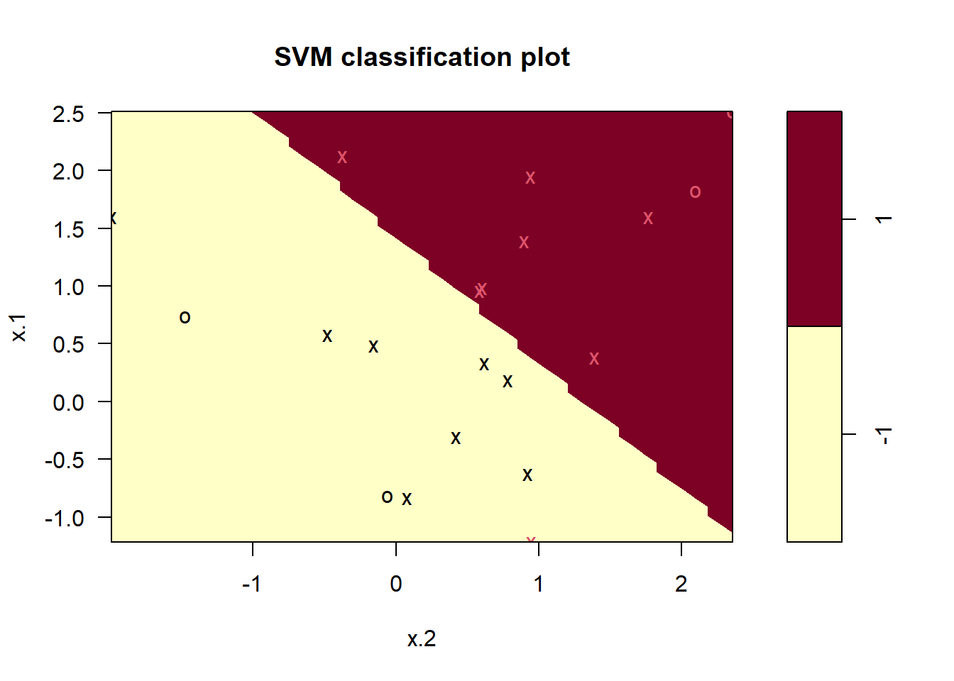
svmfit$index## [1] 1 2 3 4 5 7 9 10 12 13 14 15 16 17 18 20Now that a smaller value of the cost parameter is being used, we
obtain a larger number of support vectors, because the margin is now
wider. Unfortunately, the svm() function does not
explicitly output the coefficients of the linear decision boundary
obtained when the support vector classifier is fit, nor does it output
the width of the margin.
The e1071 library includes a built-in function,
tune(), to perform cross-validation. By default,
tune() performs ten-fold cross-validation on a set of
models of interest. In order to use this function, we pass in relevant
information about the set of models that are under consideration. The
following command indicates that we want to compare SVMs with a linear
kernel, using a range of values of the cost parameter.
set.seed(1)
tune.out <- tune(svm, y ~ ., data = dat, kernel = "linear",
    ranges = list(cost = c(0.001, 0.01, 0.1, 1, 5, 10, 100)))
We can easily access the cross-validation errors for each of these
models using the summary() command:
summary(tune.out)##
## Parameter tuning of 'svm':
##
## - sampling method: 10-fold cross validation
##
## - best parameters:
## cost
## 0.1
##
## - best performance: 0.05
##
## - Detailed performance results:
## cost error dispersion
## 1 1e-03 0.55 0.4377975
## 2 1e-02 0.55 0.4377975
## 3 1e-01 0.05 0.1581139
## 4 1e+00 0.15 0.2415229
## 5 5e+00 0.15 0.2415229
## 6 1e+01 0.15 0.2415229
## 7 1e+02 0.15 0.2415229We see that cost = 0.1 results in the lowest
cross-validation error rate. The tune() function stores the
best model obtained, which can be accessed as follows:
bestmod <- tune.out$best.model
summary(bestmod)
##
## Call:
## best.tune(METHOD = svm, train.x = y ~ ., data = dat, ranges = list(cost = c(0.001,
## 0.01, 0.1, 1, 5, 10, 100)), kernel = "linear")
##
##
## Parameters:
## SVM-Type: C-classification
## SVM-Kernel: linear
## cost: 0.1
##
## Number of Support Vectors: 16
##
## ( 8 8 )
##
##
## Number of Classes: 2
##
## Levels:
## -1 1The predict() function can be used to predict the class
label on a set of test observations, at any given value of the cost
parameter. We begin by generating a test data set.
xtest <- matrix(rnorm(20 * 2), ncol = 2)
ytest <- sample(c(-1, 1), 20, rep = TRUE)
xtest[ytest == 1, ] <- xtest[ytest == 1, ] + 1
testdat <- data.frame(x = xtest, y = as.factor(ytest))
Now we predict the class labels of these test observations. Here we use the best model obtained through cross-validation in order to make predictions.
ypred <- predict(bestmod, testdat)
table(predict = ypred, truth = testdat$y)
## truth
## predict -1 1
## -1 9 1
## 1 2 8Thus, with this value of cost, 17 of the test
observations are correctly classified. What if we had instead used
cost = 0.01?
svmfit <- svm(y ~ ., data = dat, kernel = "linear",
    cost = .01, scale = FALSE)
ypred <- predict(svmfit, testdat)
table(predict = ypred, truth = testdat$y)
## truth
## predict -1 1
## -1 11 6
## 1 0 3In this case three additional observations are misclassified.
Now consider a situation in which the two classes are linearly
separable. Then we can find a separating hyperplane using the
svm() function. We first further separate the two classes
in our simulated data so that they are linearly separable:
x[y == 1, ] <- x[y == 1, ] + 0.5
plot(x, col = (y + 5) / 2, pch = 19)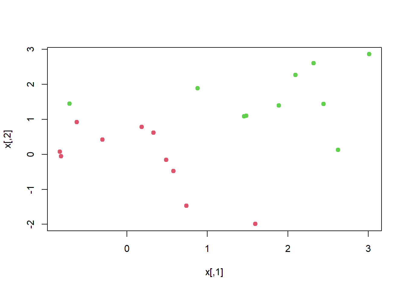
Now the observations are just barely linearly separable. We fit the
support vector classifier and plot the resulting hyperplane, using a
very large value of cost so that no observations are
misclassified.
dat <- data.frame(x = x, y = as.factor(y))
svmfit <- svm(y ~ ., data = dat, kernel = "linear",
    cost = 1e5)
summary(svmfit)
##
## Call:
## svm(formula = y ~ ., data = dat, kernel = "linear", cost = 1e+05)
##
##
## Parameters:
## SVM-Type: C-classification
## SVM-Kernel: linear
## cost: 1e+05
##
## Number of Support Vectors: 3
##
## ( 1 2 )
##
##
## Number of Classes: 2
##
## Levels:
## -1 1plot(svmfit, dat)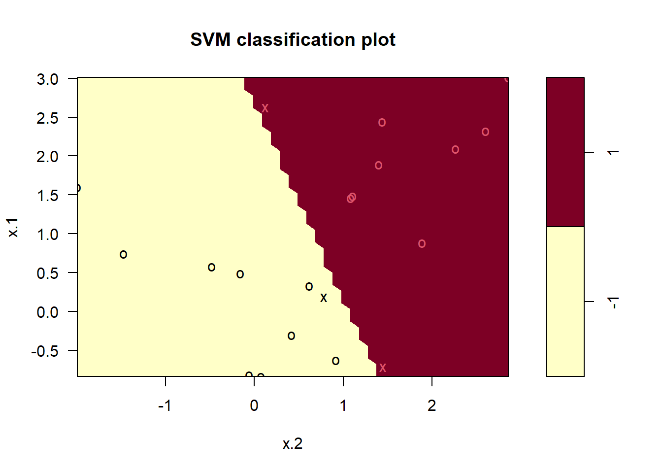
No training errors were made and only three support vectors were
used. However, we can see from the figure that the margin is very narrow
(because the observations that are not support vectors, indicated as
circles, are very close to the decision boundary). It seems likely that
this model will perform poorly on test data. We now try a smaller value
of cost:
svmfit <- svm(y ~ ., data = dat, kernel = "linear", cost = 1)
summary(svmfit)
##
## Call:
## svm(formula = y ~ ., data = dat, kernel = "linear", cost = 1)
##
##
## Parameters:
## SVM-Type: C-classification
## SVM-Kernel: linear
## cost: 1
##
## Number of Support Vectors: 7
##
## ( 4 3 )
##
##
## Number of Classes: 2
##
## Levels:
## -1 1plot(svmfit, dat)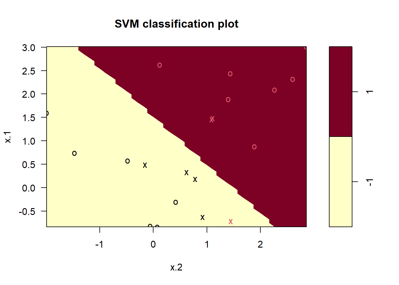
Using cost = 1, we misclassify a training observation,
but we also obtain a much wider margin and make use of seven support
vectors. It seems likely that this model will perform better on test
data than the model with cost = 1e5.
Support Vector Machine
In order to fit an SVM using a non-linear kernel, we once again use
the svm() function. However, now we use a different value
of the parameter kernel. To fit an SVM with a polynomial
kernel we use kernel = "polynomial", and to fit an SVM with
a radial kernel we use kernel = "radial". In the former
case we also use the degree argument to specify a degree
for the polynomial kernel (this is \(d\) in lecture slides), and in the latter
case we use gamma to specify a value of \(\gamma\) for the radial basis kernel.
We first generate some data with a non-linear class boundary, as follows:
set.seed(1)
x <- matrix(rnorm(200 * 2), ncol = 2)
x[1:100, ] <- x[1:100, ] + 2
x[101:150, ] <- x[101:150, ] - 2
y <- c(rep(1, 150), rep(2, 50))
dat <- data.frame(x = x, y = as.factor(y))
Plotting the data makes it clear that the class boundary is indeed non-linear:
plot(x, col = y)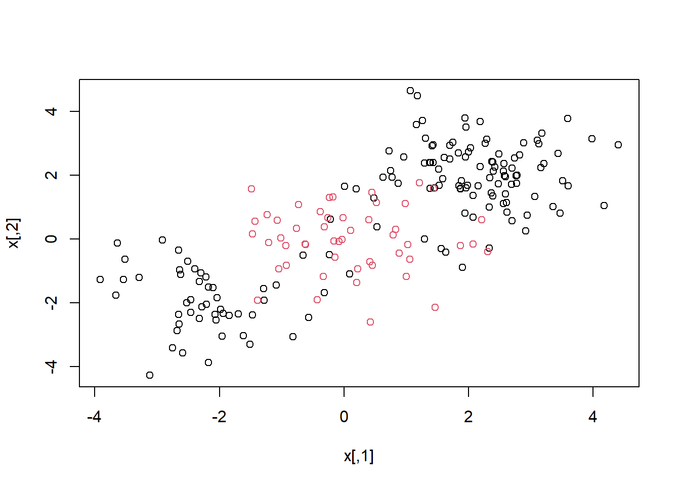
The data is randomly split into training and testing groups. We then
fit the training data using the svm() function with a
radial kernel and \(\gamma=1\):
train <- sample(200, 100)
svmfit <- svm(y ~ ., data = dat[train, ], kernel = "radial",
    gamma = 1, cost = 1)
plot(svmfit, dat[train, ])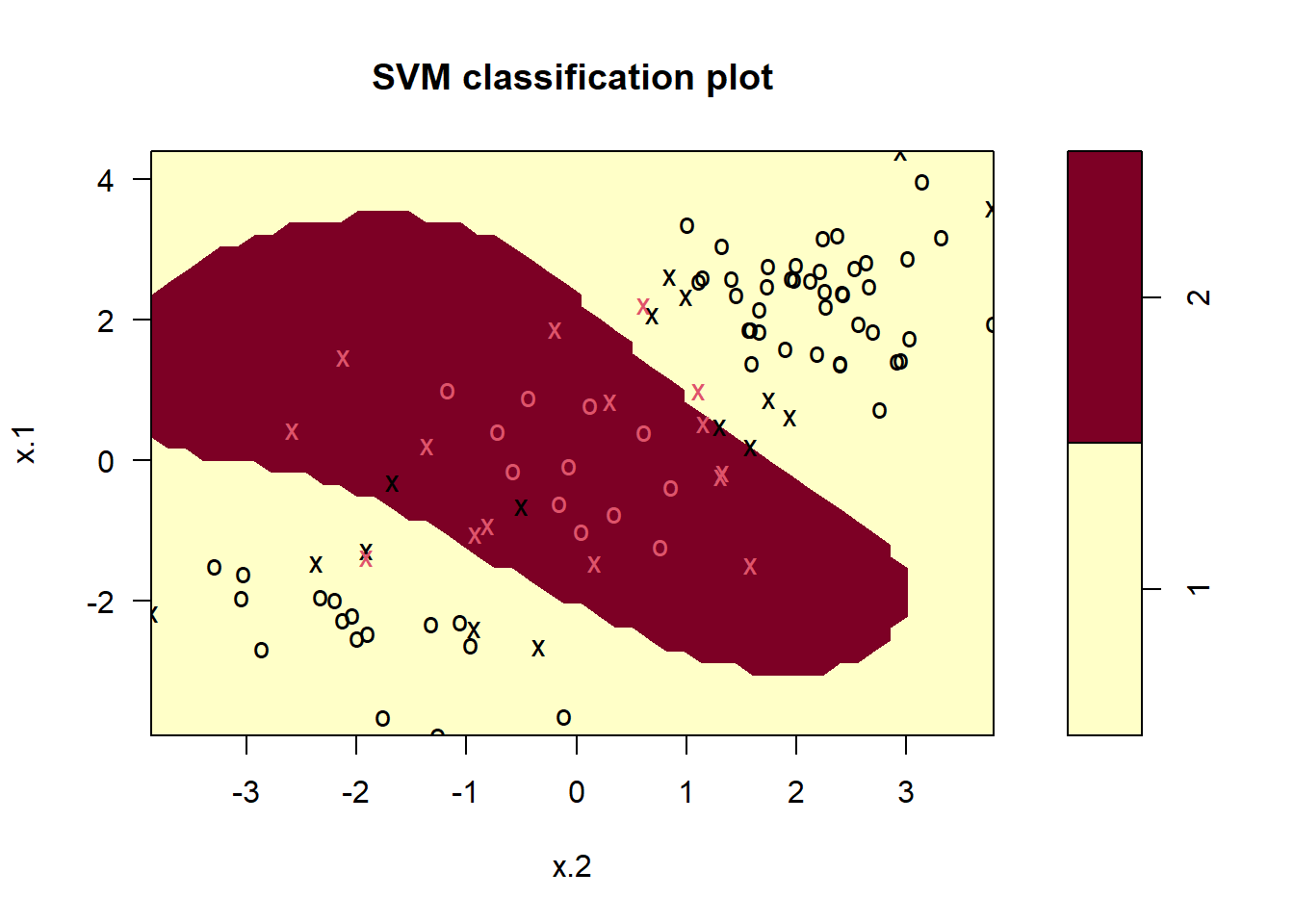
The plot shows that the resulting SVM has a decidedly non-linear
boundary. The summary() function can be used to obtain some
information about the SVM fit:
summary(svmfit)##
## Call:
## svm(formula = y ~ ., data = dat[train, ], kernel = "radial", gamma = 1,
## cost = 1)
##
##
## Parameters:
## SVM-Type: C-classification
## SVM-Kernel: radial
## cost: 1
##
## Number of Support Vectors: 31
##
## ( 16 15 )
##
##
## Number of Classes: 2
##
## Levels:
## 1 2We can see from the figure that there are a fair number of training
errors in this SVM fit. If we increase the value of cost,
we can reduce the number of training errors. However, this comes at the
price of a more irregular decision boundary that seems to be at risk of
overfitting the data.
svmfit <- svm(y ~ ., data = dat[train, ], kernel = "radial",
    gamma = 1, cost = 1e5)
plot(svmfit, dat[train, ])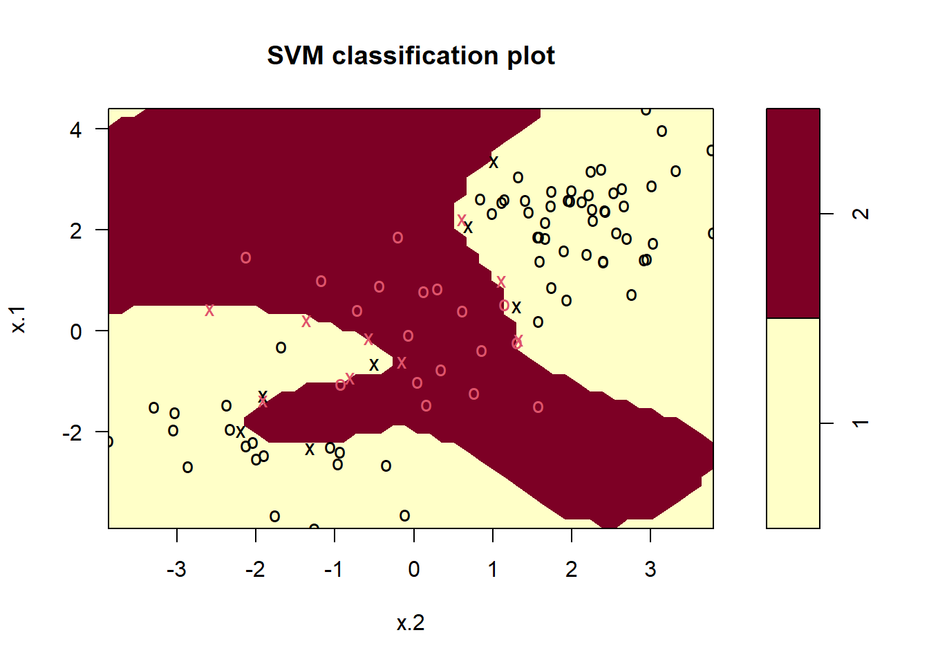
We can perform cross-validation using tune() to select
the best choice of \(\gamma\) and
cost for an SVM with a radial kernel:
set.seed(1)
tune.out <- tune(svm, y ~ ., data = dat[train, ],
    kernel = "radial",
    ranges = list(
      cost = c(0.1, 1, 10, 100, 1000),
      gamma = c(0.5, 1, 2, 3, 4)
    )
  )
summary(tune.out)
##
## Parameter tuning of 'svm':
##
## - sampling method: 10-fold cross validation
##
## - best parameters:
## cost gamma
## 1 0.5
##
## - best performance: 0.07
##
## - Detailed performance results:
## cost gamma error dispersion
## 1 1e-01 0.5 0.26 0.15776213
## 2 1e+00 0.5 0.07 0.08232726
## 3 1e+01 0.5 0.07 0.08232726
## 4 1e+02 0.5 0.14 0.15055453
## 5 1e+03 0.5 0.11 0.07378648
## 6 1e-01 1.0 0.22 0.16193277
## 7 1e+00 1.0 0.07 0.08232726
## 8 1e+01 1.0 0.09 0.07378648
## 9 1e+02 1.0 0.12 0.12292726
## 10 1e+03 1.0 0.11 0.11005049
## 11 1e-01 2.0 0.27 0.15670212
## 12 1e+00 2.0 0.07 0.08232726
## 13 1e+01 2.0 0.11 0.07378648
## 14 1e+02 2.0 0.12 0.13165612
## 15 1e+03 2.0 0.16 0.13498971
## 16 1e-01 3.0 0.27 0.15670212
## 17 1e+00 3.0 0.07 0.08232726
## 18 1e+01 3.0 0.08 0.07888106
## 19 1e+02 3.0 0.13 0.14181365
## 20 1e+03 3.0 0.15 0.13540064
## 21 1e-01 4.0 0.27 0.15670212
## 22 1e+00 4.0 0.07 0.08232726
## 23 1e+01 4.0 0.09 0.07378648
## 24 1e+02 4.0 0.13 0.14181365
## 25 1e+03 4.0 0.15 0.13540064Therefore, the best choice of parameters involves
cost = 1 and gamma = 0.5. We can view the test
set predictions for this model by applying the predict()
function to the data. Notice that to do this we subset the dataframe
dat using -train as an index set.
table(
    true = dat[-train, "y"],
    pred = predict(
      tune.out$best.model, newdata = dat[-train, ]
      )
    )
## pred
## true 1 2
## 1 67 10
## 2 2 2112% of test observations are misclassified by this SVM.
ROC Curves
The ROCR package can be used to produce ROC curves. We
first write a short function to plot an ROC curve given a vector
containing a numerical score for each observation, pred,
and a vector containing the class label for each observation,
truth.
library(ROCR)
rocplot <- function(pred, truth, ...) {
  predob <- prediction(pred, truth)
  perf <- performance(predob, "tpr", "fpr")
  plot(perf, ...)
}
SVMs and support vector classifiers output class labels for each
observation. However, it is also possible to obtain fitted
values for each observation, which are the numerical scores used to
obtain the class labels. For instance, in the case of a support vector
classifier, the fitted value for an observation \(X= (X_1, X_2, \ldots, X_p)^T\) takes the
form \(\hat{\beta}_0 + \hat{\beta}_1 X_1 +
\hat{\beta}_2 X_2 + \cdots + \hat{\beta}_p X_p\). In essence, the
sign of the fitted value determines on which side of the decision
boundary the observation lies. Therefore, the relationship between the
fitted value and the class prediction for a given observation is simple:
if the fitted value exceeds zero then the observation is assigned to one
class, and if it is less than zero then it is assigned to the other. In
order to obtain the fitted values for a given SVM model fit, we use
decision.values = TRUE when fitting svm().
Then the predict() function will output the fitted
values.
svmfit.opt <- svm(y ~ ., data = dat[train, ],
    kernel = "radial", gamma = 2, cost = 1,
    decision.values = T)
fitted <- attributes(
    predict(svmfit.opt, dat[train, ], decision.values = TRUE)
  )$decision.values
Now we can produce the ROC plot. Note we use the negative of the fitted values so that negative values correspond to class 1 and positive values to class 2.
par(mfrow = c(1, 2))
rocplot(-fitted, dat[train, "y"], main = "Training Data")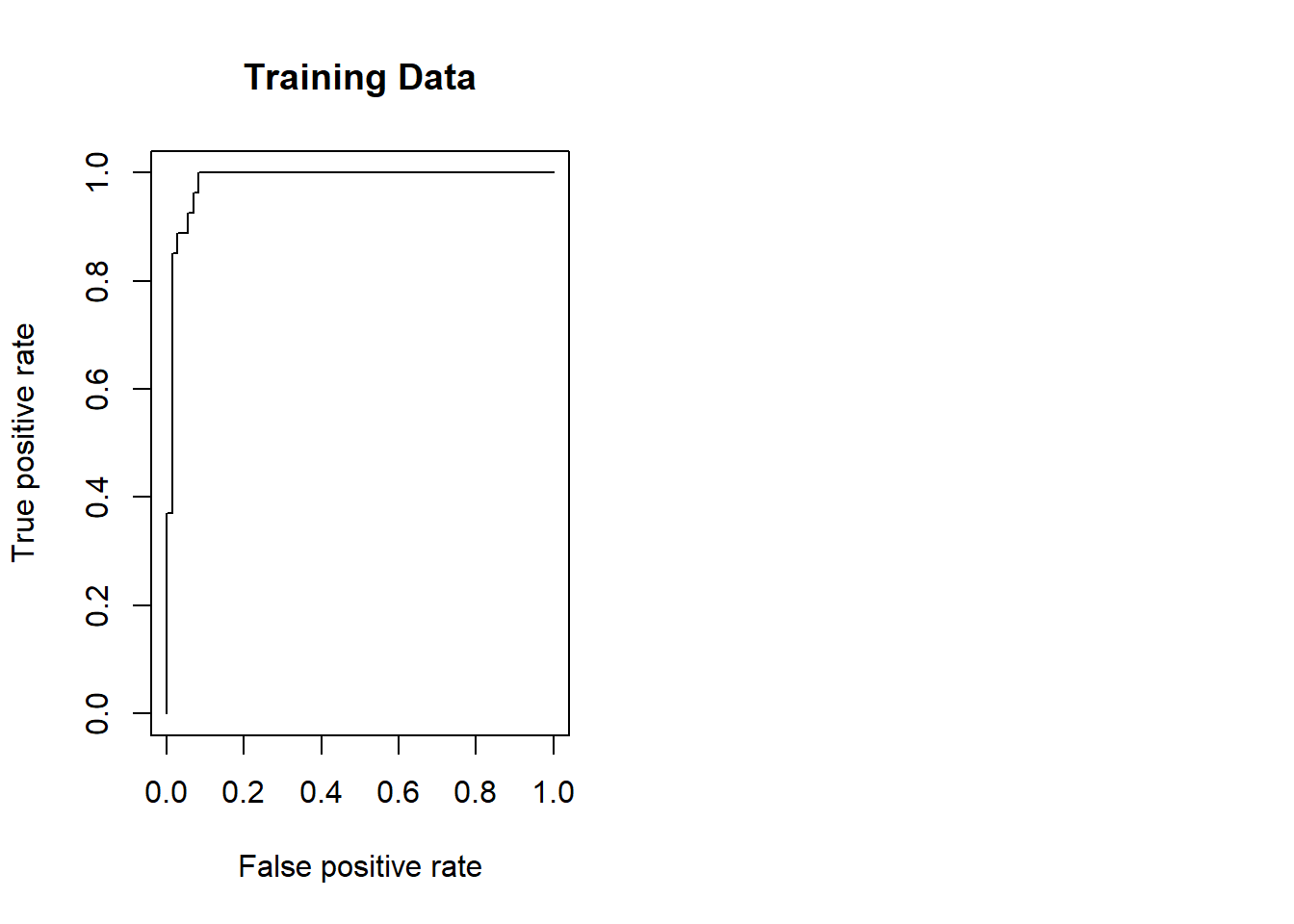
SVM appears to be producing accurate predictions. By increasing \(\gamma\) we can produce a more flexible fit and generate further improvements in accuracy.
rocplot(-fitted, dat[train, "y"], main = "Training Data")
svmfit.flex <- svm(y ~ ., data = dat[train, ],
    kernel = "radial", gamma = 50, cost = 1,
    decision.values = T)
fitted <- attributes(
    predict(svmfit.flex, dat[train, ], decision.values = T)
  )$decision.values
rocplot(-fitted, dat[train, "y"], add = T, col = "red")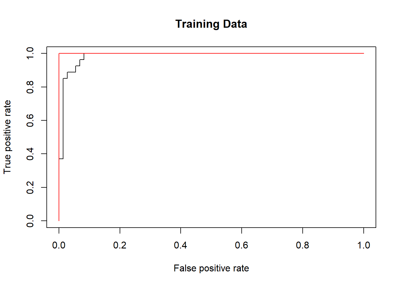
However, these ROC curves are all on the training data. We are really more interested in the level of prediction accuracy on the test data. When we compute the ROC curves on the test data, the model with \(\gamma=2\) appears to provide the most accurate results.
fitted <- attributes(
    predict(svmfit.opt, dat[-train, ], decision.values = T)
  )$decision.values
rocplot(-fitted, dat[-train, "y"], main = "Test Data")
fitted <- attributes(
    predict(svmfit.flex, dat[-train, ], decision.values = T)
  )$decision.values
rocplot(-fitted, dat[-train, "y"], add = T, col = "red")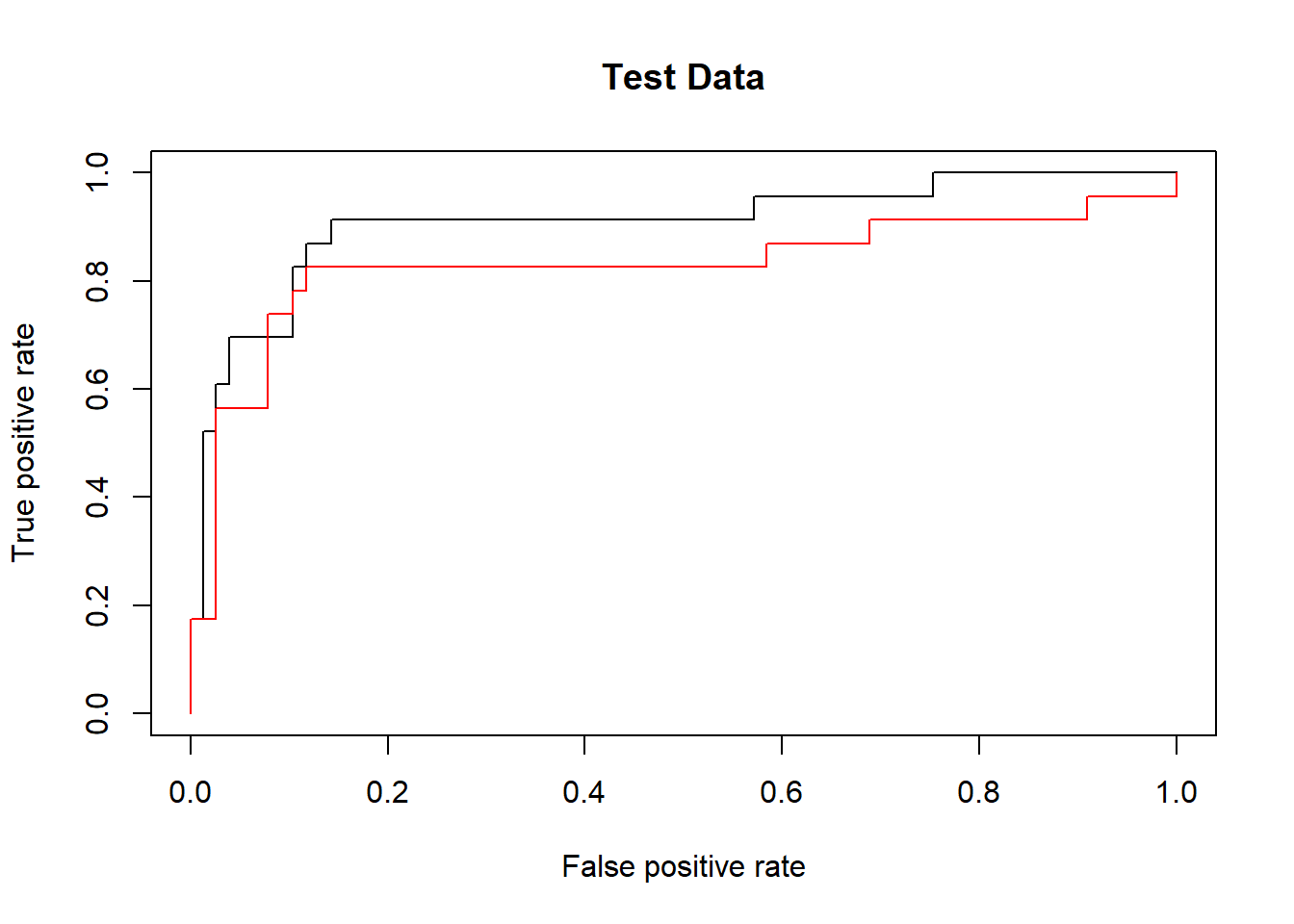
SVM with Multiple Classes
If the response is a factor containing more than two levels, then the
svm() function will perform multi-class classification
using the one-versus-one approach. We explore that setting here by
generating a third class of observations.
set.seed(1)
x <- rbind(x, matrix(rnorm(50 * 2), ncol = 2))
y <- c(y, rep(0, 50))
x[y == 0, 2] <- x[y == 0, 2] + 2
dat <- data.frame(x = x, y = as.factor(y))
par(mfrow = c(1, 1))
plot(x, col = (y + 1))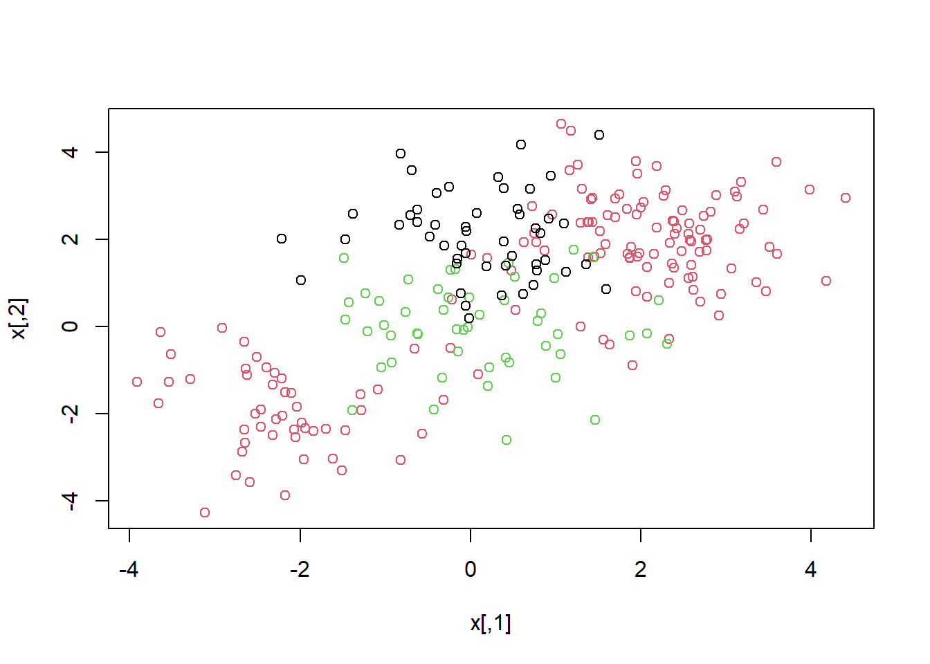
We now fit an SVM to the data:
svmfit <- svm(y ~ ., data = dat, kernel = "radial",
    cost = 10, gamma = 1)
plot(svmfit, dat)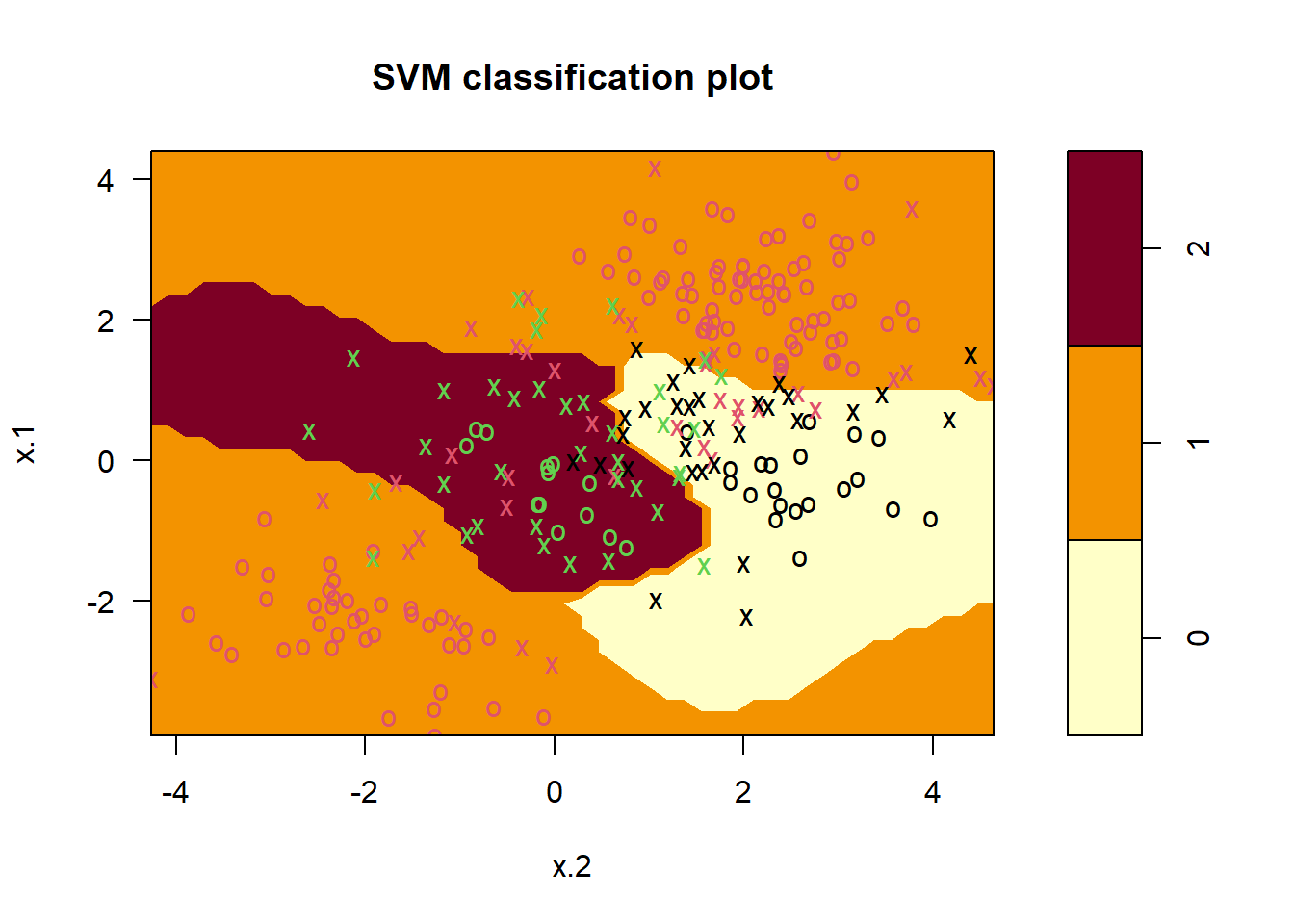
The e1071 library can also be used to perform support
vector regression, if the response vector that is passed in to
svm() is numerical rather than a factor.
Application to Gene Expression Data
We now examine the Khan data set, which consists of a
number of tissue samples corresponding to four distinct types of small
round blue cell tumors. For each tissue sample, gene expression
measurements are available. The data set consists of training data,
xtrain and ytrain, and testing data,
xtest and ytest.
We examine the dimension of the data:
library(ISLR2)
names(Khan)
## [1] "xtrain" "xtest" "ytrain" "ytest"dim(Khan$xtrain)## [1] 63 2308dim(Khan$xtest)## [1] 20 2308length(Khan$ytrain)## [1] 63length(Khan$ytest)## [1] 20This data set consists of expression measurements for 2,308 genes. The training and test sets consist of 63 and 20 observations respectively.
table(Khan$ytrain)##
## 1 2 3 4
## 8 23 12 20table(Khan$ytest)##
## 1 2 3 4
## 3 6 6 5We will use a support vector approach to predict cancer subtype using gene expression measurements. In this data set, there are a very large number of features relative to the number of observations. This suggests that we should use a linear kernel, because the additional flexibility that will result from using a polynomial or radial kernel is unnecessary.
dat <- data.frame(
    x = Khan$xtrain,
    y = as.factor(Khan$ytrain)
  )
out <- svm(y ~ ., data = dat, kernel = "linear",
    cost = 10)
summary(out)
##
## Call:
## svm(formula = y ~ ., data = dat, kernel = "linear", cost = 10)
##
##
## Parameters:
## SVM-Type: C-classification
## SVM-Kernel: linear
## cost: 10
##
## Number of Support Vectors: 58
##
## ( 20 20 11 7 )
##
##
## Number of Classes: 4
##
## Levels:
## 1 2 3 4table(out$fitted, dat$y)##
## 1 2 3 4
## 1 8 0 0 0
## 2 0 23 0 0
## 3 0 0 12 0
## 4 0 0 0 20We see that there are no training errors. In fact, this is not surprising, because the large number of variables relative to the number of observations implies that it is easy to find hyperplanes that fully separate the classes. We are most interested not in the support vector classifier’s performance on the training observations, but rather its performance on the test observations.
dat.te <- data.frame(
    x = Khan$xtest,
    y = as.factor(Khan$ytest))
pred.te <- predict(out, newdata = dat.te)
table(pred.te, dat.te$y)
##
## pred.te 1 2 3 4
## 1 3 0 0 0
## 2 0 6 2 0
## 3 0 0 4 0
## 4 0 0 0 5We see that using cost = 10 yields two test set errors
on this data.