Unsupervised Learning I - Clustering Analysis

References

Chapter 12.5.3, [ISLR2] An Introduction to Statistical Learning - with Applications in R (2nd Edition). Free access to download the book: https://www.statlearning.com/

To see the help file of a function funcname, type ?funcname.

K-Means Clustering

The function kmeans() performs K-means clustering in R. We begin with a simple simulated example in which there truly are two clusters in the data: the first 25 observations have a mean shift relative to the next 25 observations.

set.seed(1)
x <- matrix(rnorm(50 * 2), ncol = 2)
x[1:25, 1] <- x[1:25, 1] + 3
x[1:25, 2] <- x[1:25, 2] - 4

We now perform K-means clustering with K=2.

km.out <- kmeans(x, 2, nstart = 20)

The cluster assignments of the 50 observations are contained in km.out$cluster.

km.out$cluster

##  [1] 1 1 1 1 1 1 1 1 1 1 1 1 1 1 1 1 1 1 1 1 1 1 1 1 1 2 2 2 2 2 2 2 2 2 2 2 2 2
## [39] 2 2 2 2 2 2 2 2 2 2 2 2

The K-means clustering perfectly separated the observations into two clusters even though we did not supply any group information to kmeans(). We can plot the data, with each observation colored according to its cluster assignment.

#par(mfrow = c(1, 2))
plot(x, col = (km.out$cluster + 1),
    main = "K-Means Clustering Results with K = 2",
    xlab = "", ylab = "", pch = 20, cex = 2)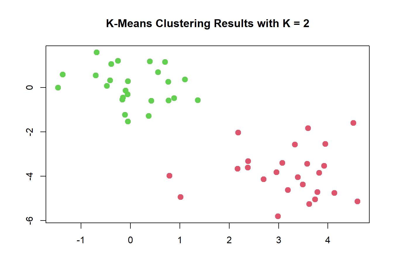

In this example, we knew that there really were two clusters because we generated the data. However, for real data, in general we do not know the true number of clusters. We could instead have performed K-means clustering on this example with K=3.

set.seed(2)
km.out <- kmeans(x, 3, nstart = 20)
km.out

## K-means clustering with 3 clusters of sizes 20, 25, 5
## 
## Cluster means:
##         [,1]        [,2]
## 1 3.08290361 -4.26589906
## 2 0.03223135  0.06924384
## 3 3.51171162 -2.10935842
## 
## Clustering vector:
##  [1] 1 1 1 1 3 3 1 1 1 1 3 1 1 1 1 1 1 3 1 3 1 1 1 1 1 2 2 2 2 2 2 2 2 2 2 2 2 2
## [39] 2 2 2 2 2 2 2 2 2 2 2 2
## 
## Within cluster sum of squares by cluster:
## [1] 27.901401 28.534174  3.740301
##  (between_SS / total_SS =  84.7 %)
## 
## Available components:
## 
## [1] "cluster"      "centers"      "totss"        "withinss"     "tot.withinss"
## [6] "betweenss"    "size"         "iter"         "ifault"

plot(x, col = (km.out$cluster + 1),
    main = "K-Means Clustering Results with K = 3",
    xlab = "", ylab = "", pch = 20, cex = 2)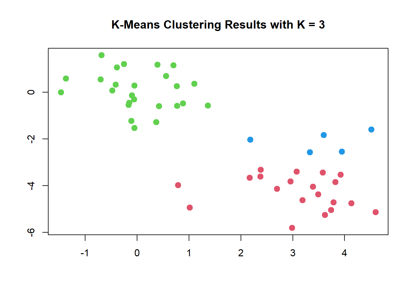

When K=3, K-means clustering splits up the two clusters.

To run the kmeans() function in R with multiple initial cluster assignments, we use the nstart argument. If a value of nstart greater than one is used, then K-means clustering will be performed using multiple random assignments in Step 1 of K-means Clustering Algorithm, and the kmeans() function will report only the best results. Here we compare using nstart = 1 to nstart = 20.

set.seed(3)
km.out <- kmeans(x, 3, nstart = 1)
km.out$tot.withinss

## [1] 60.17588

km.out <- kmeans(x, 3, nstart = 20)
km.out$tot.withinss

## [1] 60.17588

Note that km.out$tot.withinss is the total within-cluster sum of squares, which we seek to minimize by performing K-means clustering. The individual within-cluster sum-of-squares are contained in the vector km.out$withinss.

We strongly recommend always running K-means clustering with a large value of nstart, such as 20 or 50, since otherwise an undesirable local optimum may be obtained.

When performing K-means clustering, in addition to using multiple initial cluster assignments, it is also important to set a random seed using the set.seed() function. This way, the initial cluster assignments in Step 1 can be replicated, and the K-means output will be fully reproducible.

Hierarchical Clustering

The hclust() function implements hierarchical clustering in R. In the following example we use the simulated data before to plot the hierarchical clustering dendrogram using complete, single, and average linkage clustering, with Euclidean distance as the dissimilarity measure.

We begin by clustering observations using complete linkage. The dist() function is used to compute the $50 \times 50$ inter-observation Euclidean distance matrix.

hc.complete <- hclust(dist(x), method = "complete")

We could just as easily perform hierarchical clustering with average or single linkage instead:

hc.average <- hclust(dist(x), method = "average")
hc.single <- hclust(dist(x), method = "single")

We can now plot the dendrograms obtained using the usual plot() function. The numbers at the bottom of the plot identify each observation.

par(mfrow = c(1, 3))
plot(hc.complete, main = "Complete Linkage",
    xlab = "", sub = "", cex = .9)
plot(hc.average, main = "Average Linkage",
    xlab = "", sub = "", cex = .9)
plot(hc.single, main = "Single Linkage",
    xlab = "", sub = "", cex = .9)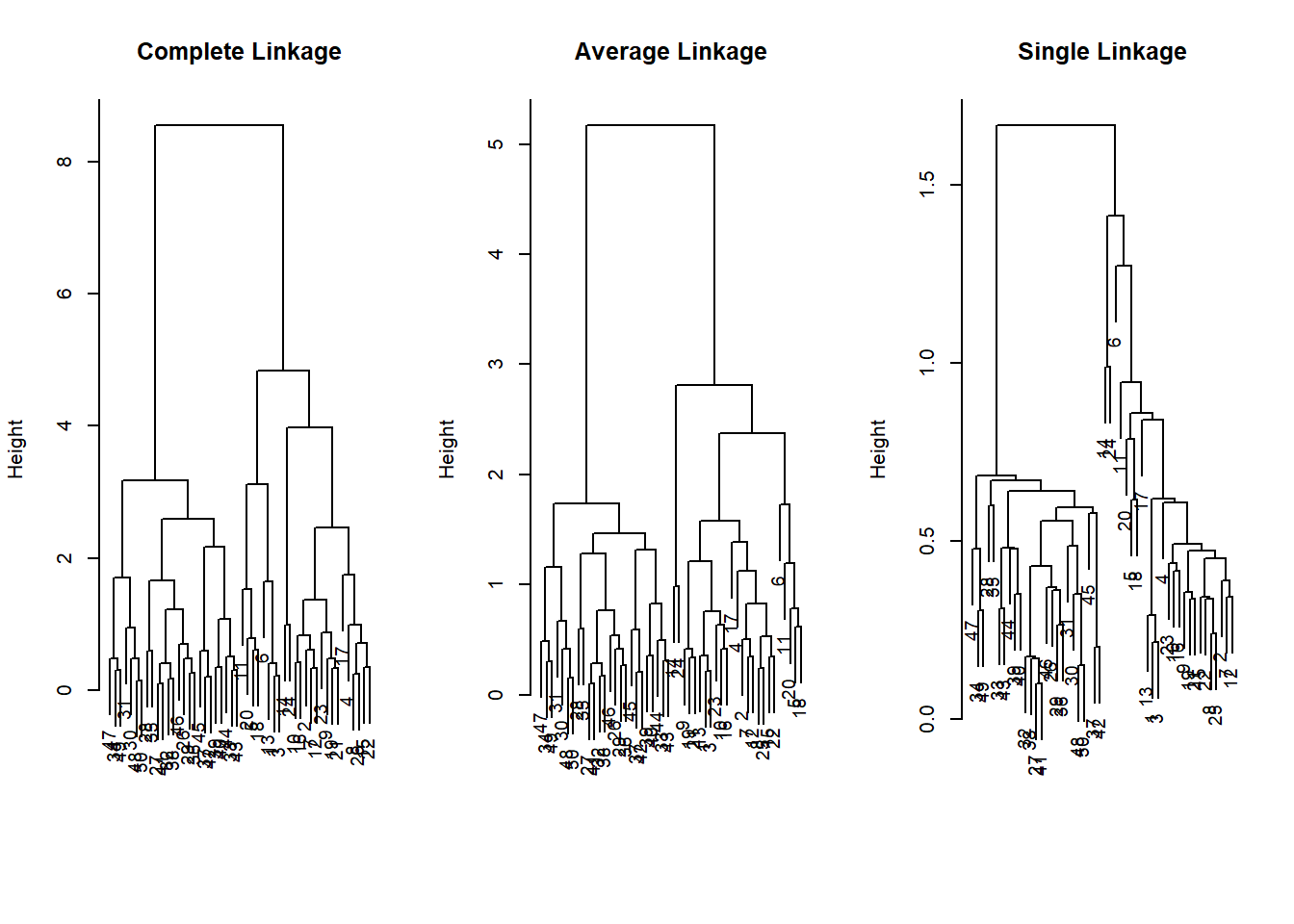

To determine the cluster labels for each observation associated with a given cut of the dendrogram, we can use the cutree() function:

cutree(hc.complete, 2)

##  [1] 1 1 1 1 1 1 1 1 1 1 1 1 1 1 1 1 1 1 1 1 1 1 1 1 1 2 2 2 2 2 2 2 2 2 2 2 2 2
## [39] 2 2 2 2 2 2 2 2 2 2 2 2

cutree(hc.average, 2)

##  [1] 1 1 1 1 1 1 1 1 1 1 1 1 1 1 1 1 1 1 1 1 1 1 1 1 1 2 2 2 2 2 2 2 2 2 2 2 2 2
## [39] 2 2 2 2 2 2 2 2 2 2 2 2

cutree(hc.single, 2)

##  [1] 1 1 1 1 1 1 1 1 1 1 1 1 1 1 1 1 1 1 1 1 1 1 1 1 1 2 2 2 2 2 2 2 2 2 2 2 2 2
## [39] 2 2 2 2 2 2 2 2 2 2 2 2

The second argument to cutree() is the number of clusters we wish to obtain.

For this data, complete and average linkage generally separate the observations into their correct groups. However, single linkage identifies one point as belonging to its own cluster. A more sensible answer is obtained when four clusters are selected, although there are still two singletons.

cutree(hc.single, 4)

##  [1] 1 1 1 1 1 2 1 1 1 1 1 1 1 3 1 1 1 1 1 1 1 1 1 3 1 4 4 4 4 4 4 4 4 4 4 4 4 4
## [39] 4 4 4 4 4 4 4 4 4 4 4 4

To scale the variables before performing hierarchical clustering of the observations, we use the scale() function:

xsc <- scale(x)
plot(hclust(dist(xsc), method = "complete"),
    main = "Hierarchical Clustering with Scaled Features")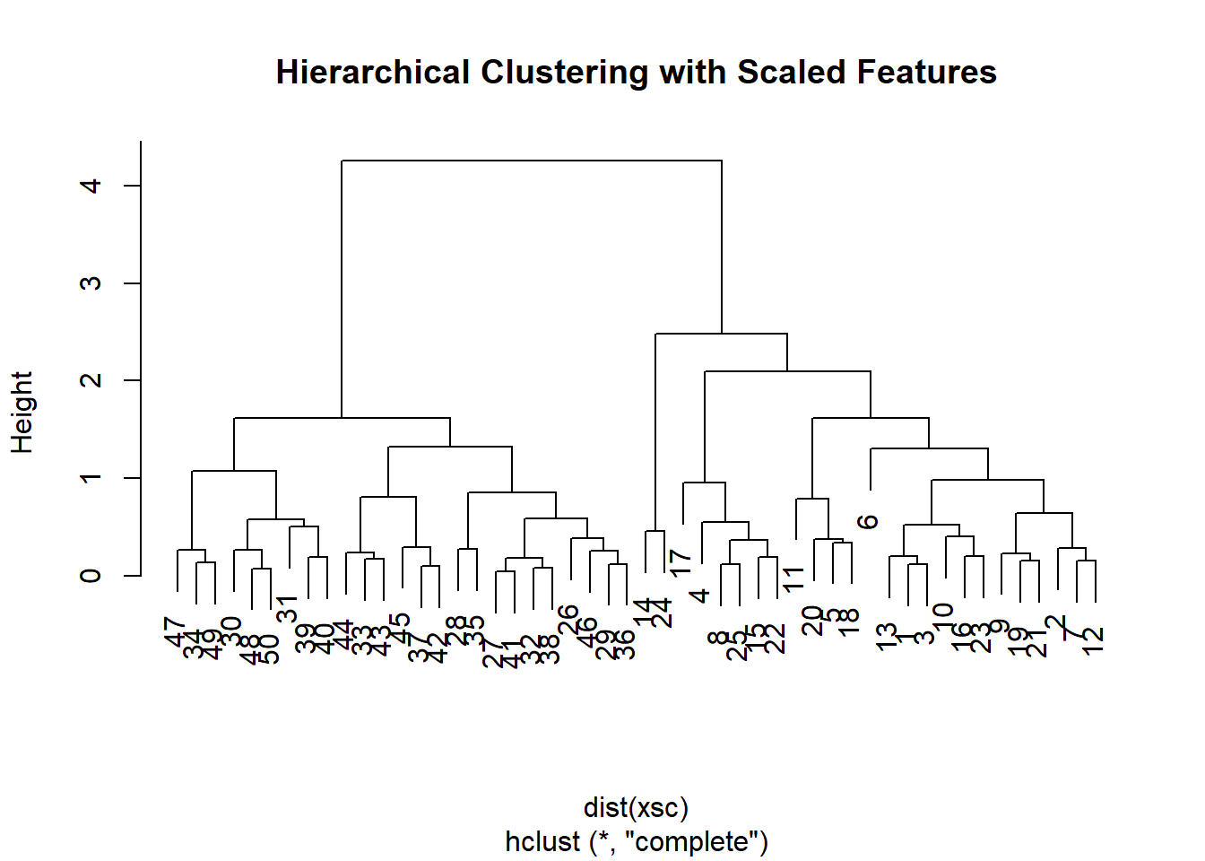

Correlation-based distance can be computed using the as.dist() function, which converts an arbitrary square symmetric matrix into a form that the hclust() function recognizes as a distance matrix. However, this only makes sense for data with at least three features since the absolute correlation between any two observations with measurements on two features is always 1. Hence, we will cluster a three-dimensional data set. This data set does not contain any true clusters.

x <- matrix(rnorm(30 * 3), ncol = 3)
dd <- as.dist(sqrt((1 - cor(t(x)))/2))
plot(hclust(dd, method = "complete"),
    main = "Complete Linkage with Correlation-Based Distance",
    xlab = "", sub = "")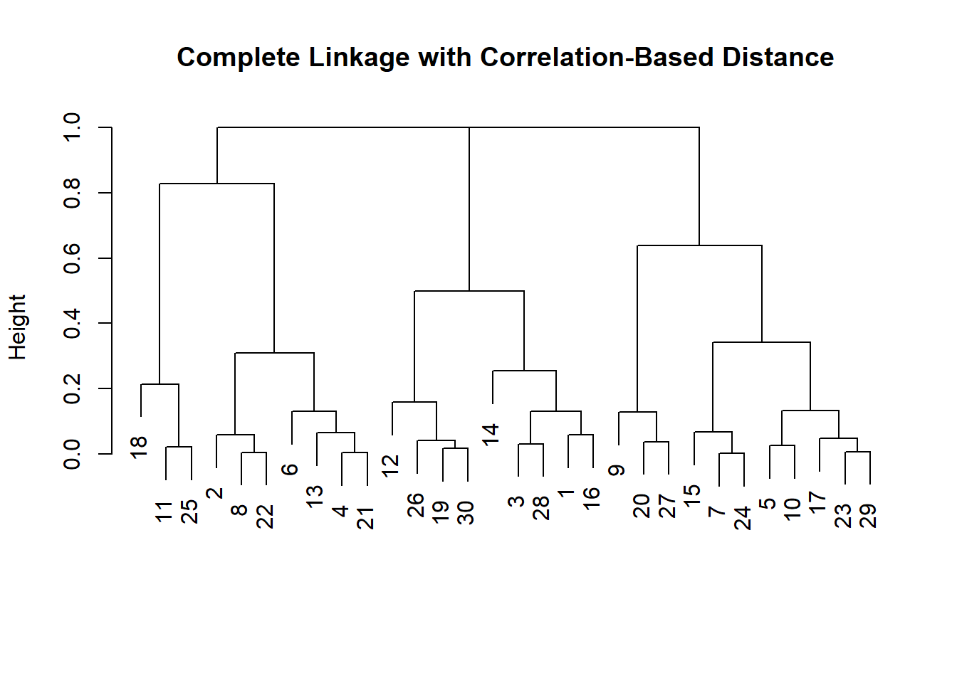

NCI60 Data Example

Unsupervised techniques are often used in the analysis of genomic data. In particular, clustering and PCA are popular tools. We illustrate these techniques on the NCI cancer cell line microarray data, which consists of 6,830 gene expression measurements on 64 cancer cell lines.

library(ISLR2)
nci.labs <- NCI60$labs
nci.data <- NCI60$data

Each cell line is labeled with a cancer type, given in nci.labs. We do not make use of the cancer types in performing clustering/PCA, as these are unsupervised techniques. But after performing clustering/PCA, we will check to see the extent to which these cancer types agree with the results of these unsupervised techniques.

The data has 64 rows and 6,830 columns.

dim(nci.data)

## [1]   64 6830

We begin by examining the cancer types for the cell lines.

nci.labs[1:4]

## [1] "CNS"   "CNS"   "CNS"   "RENAL"

table(nci.labs)

## nci.labs
##      BREAST         CNS       COLON K562A-repro K562B-repro    LEUKEMIA 
##           7           5           7           1           1           6 
## MCF7A-repro MCF7D-repro    MELANOMA       NSCLC     OVARIAN    PROSTATE 
##           1           1           8           9           6           2 
##       RENAL     UNKNOWN 
##           9           1

Clustering the Observations of the NCI60 Data

We now proceed to hierarchically cluster the cell lines in the NCI data, with the goal of finding out whether or not the observations cluster into distinct types of cancer. To begin, we standardize the variables to have mean zero and standard deviation one. As mentioned earlier, this step is optional and should be performed only if we want each gene to be on the same scale.

sd.data <- scale(nci.data)

We now perform hierarchical clustering of the observations using complete, single, and average linkage. Euclidean distance is used as the dissimilarity measure.

par(mfrow = c(1, 3))
data.dist <- dist(sd.data)
plot(hclust(data.dist), xlab = "", sub = "", ylab = "",
    labels = nci.labs, main = "Complete Linkage")
plot(hclust(data.dist, method = "average"),
    labels = nci.labs, main = "Average Linkage",
    xlab = "", sub = "", ylab = "")
plot(hclust(data.dist, method = "single"),
    labels = nci.labs,  main = "Single Linkage",
    xlab = "", sub = "", ylab = "")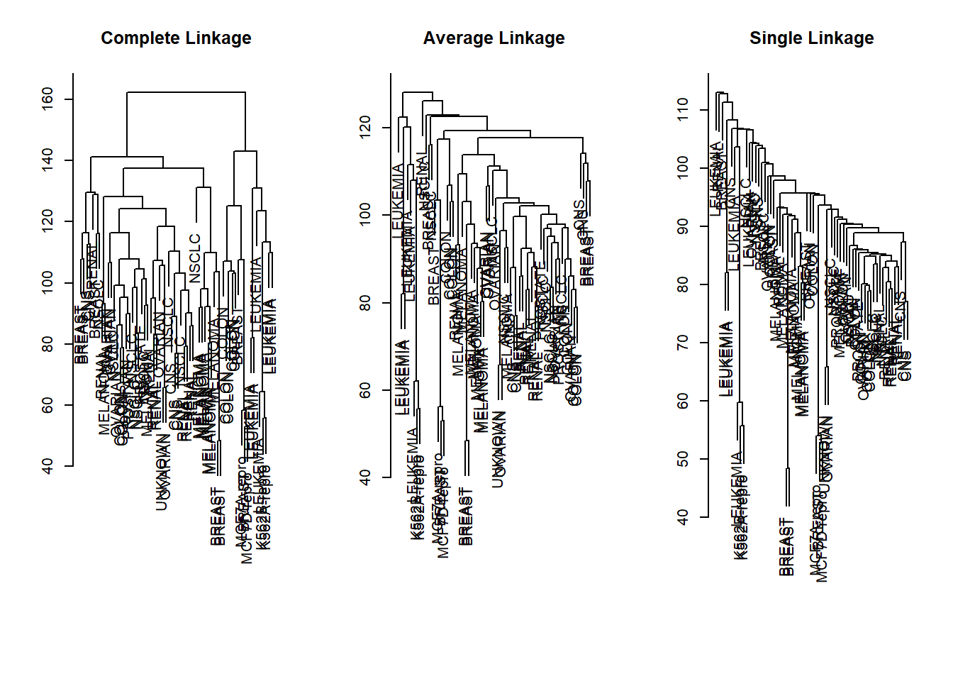

We see that the choice of linkage certainly does affect the results obtained. Typically, single linkage will tend to yield trailing clusters: very large clusters onto which individual observations attach one-by-one. On the other hand, complete and average linkage tend to yield more balanced, attractive clusters. For this reason, complete and average linkage are generally preferred to single linkage. Clearly cell lines within a single cancer type do tend to cluster together, although the clustering is not perfect. We will use complete linkage hierarchical clustering for the analysis that follows.

We can cut the dendrogram at the height that will yield a particular number of clusters, say four:

hc.out <- hclust(dist(sd.data))
hc.clusters <- cutree(hc.out, 4)
table(hc.clusters, nci.labs)

##            nci.labs
## hc.clusters BREAST CNS COLON K562A-repro K562B-repro LEUKEMIA MCF7A-repro
##           1      2   3     2           0           0        0           0
##           2      3   2     0           0           0        0           0
##           3      0   0     0           1           1        6           0
##           4      2   0     5           0           0        0           1
##            nci.labs
## hc.clusters MCF7D-repro MELANOMA NSCLC OVARIAN PROSTATE RENAL UNKNOWN
##           1           0        8     8       6        2     8       1
##           2           0        0     1       0        0     1       0
##           3           0        0     0       0        0     0       0
##           4           1        0     0       0        0     0       0

There are some clear patterns. All the leukemia cell lines fall in cluster 3, while the breast cancer cell lines are spread out over three different clusters. We can plot the cut on the dendrogram that produces these four clusters:

par(mfrow = c(1, 1))
plot(hc.out, labels = nci.labs)
abline(h = 139, col = "red")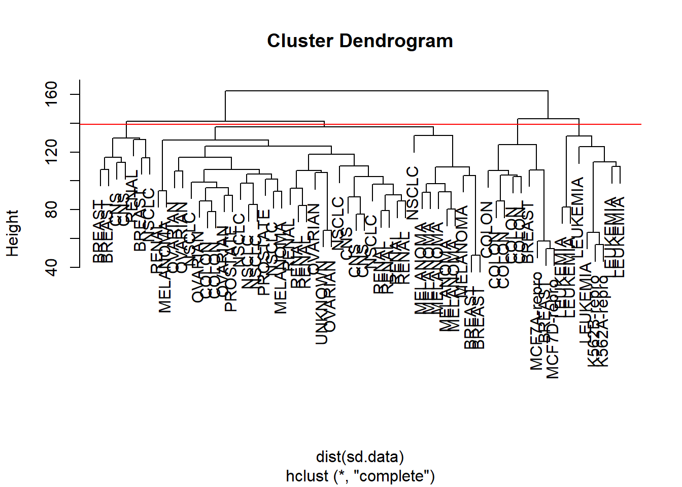

The abline() function draws a straight line on top of any existing plot in R. The argument h = 139 plots a horizontal line at height 139 on the dendrogram; this is the height that results in four distinct clusters. It is easy to verify that the resulting clusters are the same as the ones we obtained using cutree(hc.out, 4).

Printing the output of hclust gives a useful brief summary of the object:

hc.out

## 
## Call:
## hclust(d = dist(sd.data))
## 
## Cluster method   : complete 
## Distance         : euclidean 
## Number of objects: 64

We claimed earlier that K-means clustering and hierarchical clustering with the dendrogram cut to obtain the same number of clusters can yield very different results. How do these NCI hierarchical clustering results compare to what we get if we perform K-means clustering with K=4?

set.seed(2)
km.out <- kmeans(sd.data, 4, nstart = 20)
km.clusters <- km.out$cluster
table(km.clusters, hc.clusters)

##            hc.clusters
## km.clusters  1  2  3  4
##           1 11  0  0  9
##           2 20  7  0  0
##           3  9  0  0  0
##           4  0  0  8  0