Unsupervised Learning II - Dimension Reduction
Patrick PUN Chi Seng (NTU Sg)
References
Chapter 12.5.1, [ISLR2] An Introduction to Statistical Learning - with Applications in R (2nd Edition). Free access to download the book: https://www.statlearning.com/
To see the help file of a function funcname, type
?funcname.
Principal Component Analysis
We perform PCA on the USArrests data set, which is part
of the base R package.
The rows of the data set contain the 50 states, in alphabetical order.
states <- row.names(USArrests)
states
## [1] "Alabama" "Alaska" "Arizona" "Arkansas"
## [5] "California" "Colorado" "Connecticut" "Delaware"
## [9] "Florida" "Georgia" "Hawaii" "Idaho"
## [13] "Illinois" "Indiana" "Iowa" "Kansas"
## [17] "Kentucky" "Louisiana" "Maine" "Maryland"
## [21] "Massachusetts" "Michigan" "Minnesota" "Mississippi"
## [25] "Missouri" "Montana" "Nebraska" "Nevada"
## [29] "New Hampshire" "New Jersey" "New Mexico" "New York"
## [33] "North Carolina" "North Dakota" "Ohio" "Oklahoma"
## [37] "Oregon" "Pennsylvania" "Rhode Island" "South Carolina"
## [41] "South Dakota" "Tennessee" "Texas" "Utah"
## [45] "Vermont" "Virginia" "Washington" "West Virginia"
## [49] "Wisconsin" "Wyoming"The columns of the data set contain the four variables.
names(USArrests)## [1] "Murder" "Assault" "UrbanPop" "Rape"We first briefly examine the data. We notice that the variables have vastly different means.
apply(USArrests, 2, mean)## Murder Assault UrbanPop Rape
## 7.788 170.760 65.540 21.232Note that the apply() function allows us to apply a
function—in this case, the mean() function—to each row or
column of the data set. The second input here denotes whether we wish to
compute the mean of the rows, 1, or the columns, 2. We see that there
are on average three times as many rapes as murders, and more than eight
times as many assaults as rapes.
We can also examine the variances of the four variables using the
apply() function.
apply(USArrests, 2, var)## Murder Assault UrbanPop Rape
## 18.97047 6945.16571 209.51878 87.72916Not surprisingly, the variables also have vastly different variances:
the UrbanPop variable measures the percentage of the
population in each state living in an urban area, which is not a
comparable number to the number of rapes in each state per 100,000
individuals. If we failed to scale the variables before performing PCA,
then most of the principal components that we observed would be driven
by the Assault variable, since it has by far the largest
mean and variance. Thus, it is important to standardize the variables to
have mean zero and standard deviation one before performing PCA.
We now perform principal components analysis using the
prcomp() function, which is one of several functions in
R that perform PCA.
pr.out <- prcomp(USArrests, scale = TRUE)By default, the prcomp() function centers the variables
to have mean zero. By using the option scale = TRUE, we
scale the variables to have standard deviation one. The output from
prcomp() contains a number of useful quantities.
names(pr.out)## [1] "sdev" "rotation" "center" "scale" "x"The center and scale components correspond
to the means and standard deviations of the variables that were used for
scaling prior to implementing PCA.
pr.out$center## Murder Assault UrbanPop Rape
## 7.788 170.760 65.540 21.232pr.out$scale## Murder Assault UrbanPop Rape
## 4.355510 83.337661 14.474763 9.366385The rotation matrix provides the principal component
loadings; each column of pr.out$rotation contains the
corresponding principal component loading vector.\footnote{This function
names it the rotation matrix, because when we matrix-multiply the \(\bf X\) matrix by
pr.out$rotation, it gives us the coordinates of the data in
the rotated coordinate system. These coordinates are the principal
component scores.}
pr.out$rotation## PC1 PC2 PC3 PC4
## Murder -0.5358995 -0.4181809 0.3412327 0.64922780
## Assault -0.5831836 -0.1879856 0.2681484 -0.74340748
## UrbanPop -0.2781909 0.8728062 0.3780158 0.13387773
## Rape -0.5434321 0.1673186 -0.8177779 0.08902432We see that there are four distinct principal components. This is to be expected because there are in general \(\min(n-1,p)\) informative principal components in a data set with \(n\) observations and \(p\) variables.
Using the prcomp() function, we do not need to
explicitly multiply the data by the principal component loading vectors
in order to obtain the principal component score vectors. Rather the
\(50 \times 4\) matrix x
has as its columns the principal component score vectors. That is, the
\(k\)th column is the \(k\)th principal component score vector.
dim(pr.out$x)## [1] 50 4We can plot the first two principal components as follows:
biplot(pr.out, scale = 0)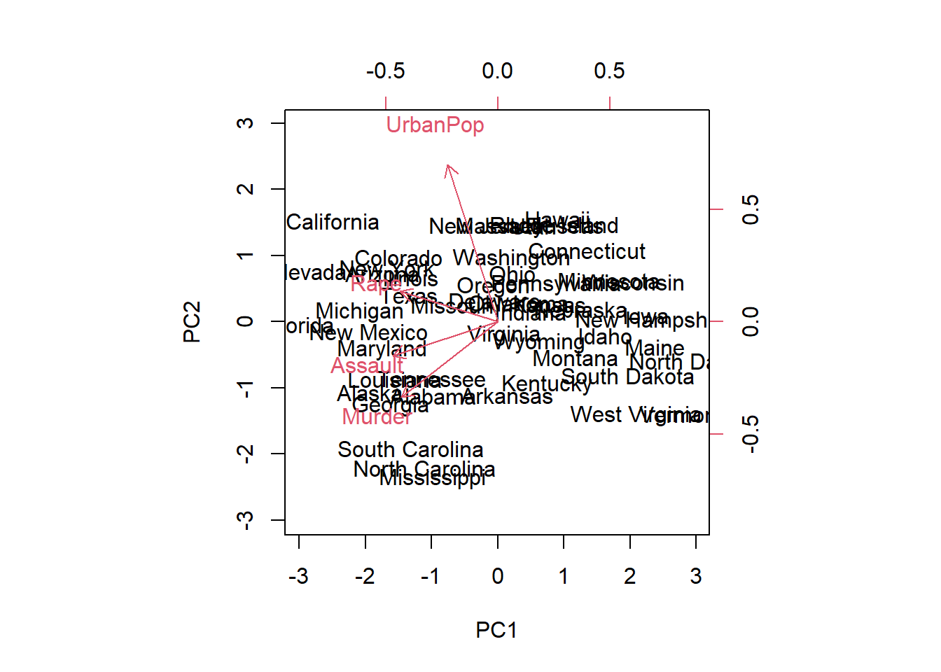
The scale = 0 argument to biplot() ensures
that the arrows are scaled to represent the loadings; other values for
scale give slightly different biplots with different
interpretations.
The prcomp() function also outputs the standard
deviation of each principal component. For instance, on the
USArrests data set, we can access these standard deviations
as follows:
pr.out$sdev## [1] 1.5748783 0.9948694 0.5971291 0.4164494The variance explained by each principal component is obtained by squaring these:
pr.var <- pr.out$sdev^2
pr.var
## [1] 2.4802416 0.9897652 0.3565632 0.1734301To compute the proportion of variance explained by each principal component, we simply divide the variance explained by each principal component by the total variance explained by all four principal components:
pve <- pr.var / sum(pr.var)
pve
## [1] 0.62006039 0.24744129 0.08914080 0.04335752We see that the first principal component explains 62.0% of the variance in the data, the next principal component explains 24.7% of the variance, and so forth. We can plot the PVE explained by each component, as well as the cumulative PVE, as follows:
par(mfrow = c(1, 2))
plot(pve, xlab = "Principal Component",
    ylab = "Proportion of Variance Explained", ylim = c(0, 1),
    type = "b")
plot(cumsum(pve), xlab = "Principal Component",
    ylab = "Cumulative Proportion of Variance Explained",
    ylim = c(0, 1), type = "b")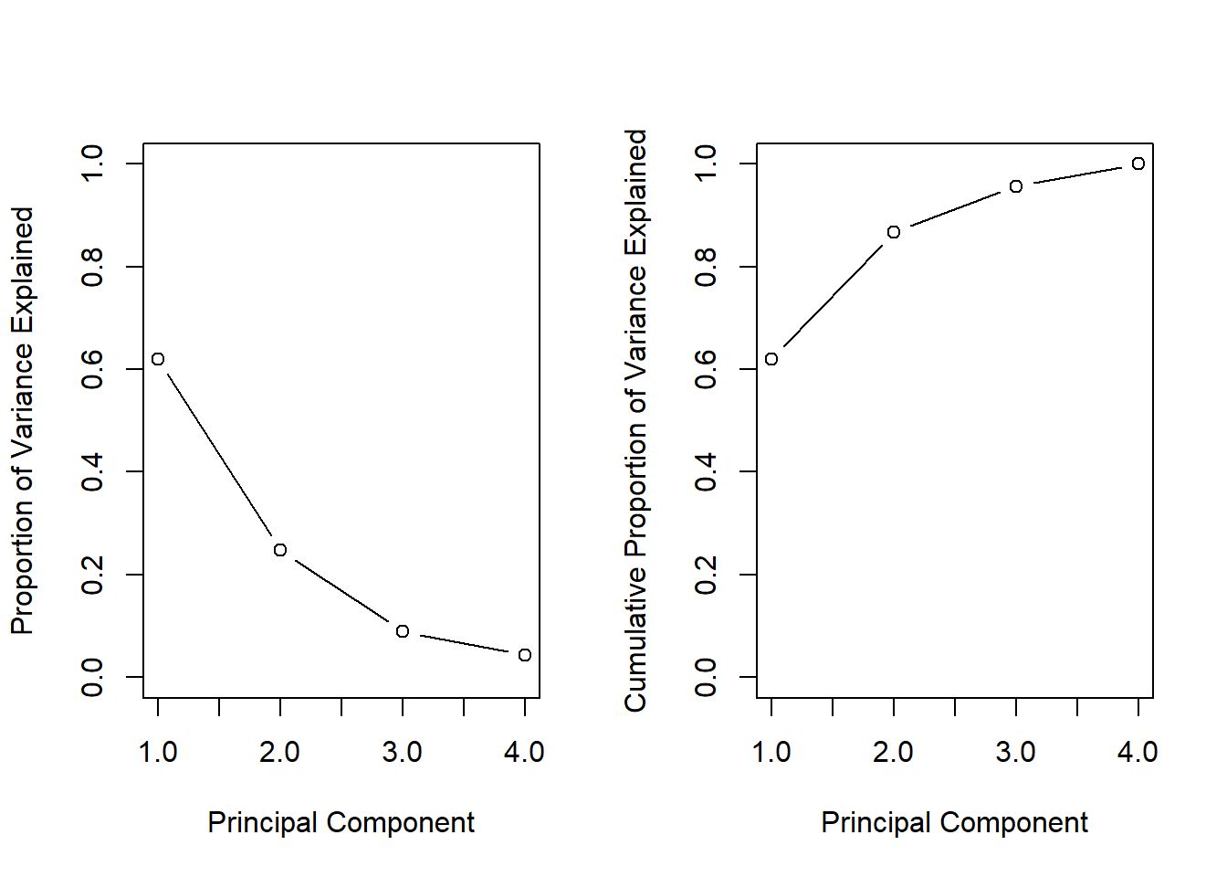
On a related note, one can verify the PCA results using eigendecomposition:
eigen.out=eigen(cov(scale(USArrests))); eigen.out## eigen() decomposition
## $values
## [1] 2.4802416 0.9897652 0.3565632 0.1734301
##
## $vectors
## [,1] [,2] [,3] [,4]
## [1,] -0.5358995 0.4181809 -0.3412327 0.64922780
## [2,] -0.5831836 0.1879856 -0.2681484 -0.74340748
## [3,] -0.2781909 -0.8728062 -0.3780158 0.13387773
## [4,] -0.5434321 -0.1673186 0.8177779 0.08902432# eigen.out=eigen(cor(USArrests)); eigen.out
sqrt(eigen.out$values)## [1] 1.5748783 0.9948694 0.5971291 0.4164494PCA on the NCI60 Data
We illustrate the PCA on the NCI cancer cell line
microarray data, which consists of 6,830 gene expression measurements on
64 cancer cell lines.
library(ISLR2)
nci.labs <- NCI60$labs
nci.data <- NCI60$data
We first perform PCA on the data after scaling the variables (genes) to have standard deviation one, although one could reasonably argue that it is better not to scale the genes.
pr.out <- prcomp(nci.data, scale = TRUE)We now plot the first few principal component score vectors, in order to visualize the data. The observations (cell lines) corresponding to a given cancer type will be plotted in the same color, so that we can see to what extent the observations within a cancer type are similar to each other. We first create a simple function that assigns a distinct color to each element of a numeric vector. The function will be used to assign a color to each of the 64 cell lines, based on the cancer type to which it corresponds.
Cols <- function(vec) {
   cols <- rainbow(length(unique(vec)))
   return(cols[as.numeric(as.factor(vec))])
 }
Note that the rainbow() function takes as its argument a
positive integer, and returns a vector containing that number of
distinct colors. We now can plot the principal component score
vectors.
par(mfrow = c(1, 2))
plot(pr.out$x[, 1:2], col = Cols(nci.labs), pch = 19,
    xlab = "Z1", ylab = "Z2")
plot(pr.out$x[, c(1, 3)], col = Cols(nci.labs), pch = 19,
    xlab = "Z1", ylab = "Z3")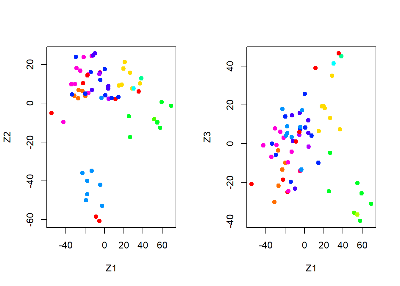
On the whole, cell lines corresponding to a single cancer type do tend to have similar values on the first few principal component score vectors. This indicates that cell lines from the same cancer type tend to have pretty similar gene expression levels.
We can obtain a summary of the proportion of variance explained (PVE)
of the first few principal components using the summary()
method for a prcomp object (we have truncated the
printout):
summary(pr.out)## Importance of components:
## PC1 PC2 PC3 PC4 PC5 PC6
## Standard deviation 27.8535 21.48136 19.82046 17.03256 15.97181 15.72108
## Proportion of Variance 0.1136 0.06756 0.05752 0.04248 0.03735 0.03619
## Cumulative Proportion 0.1136 0.18115 0.23867 0.28115 0.31850 0.35468
## PC7 PC8 PC9 PC10 PC11 PC12
## Standard deviation 14.47145 13.54427 13.14400 12.73860 12.68672 12.15769
## Proportion of Variance 0.03066 0.02686 0.02529 0.02376 0.02357 0.02164
## Cumulative Proportion 0.38534 0.41220 0.43750 0.46126 0.48482 0.50646
## PC13 PC14 PC15 PC16 PC17 PC18
## Standard deviation 11.83019 11.62554 11.43779 11.00051 10.65666 10.48880
## Proportion of Variance 0.02049 0.01979 0.01915 0.01772 0.01663 0.01611
## Cumulative Proportion 0.52695 0.54674 0.56590 0.58361 0.60024 0.61635
## PC19 PC20 PC21 PC22 PC23 PC24
## Standard deviation 10.43518 10.3219 10.14608 10.0544 9.90265 9.64766
## Proportion of Variance 0.01594 0.0156 0.01507 0.0148 0.01436 0.01363
## Cumulative Proportion 0.63229 0.6479 0.66296 0.6778 0.69212 0.70575
## PC25 PC26 PC27 PC28 PC29 PC30 PC31
## Standard deviation 9.50764 9.33253 9.27320 9.0900 8.98117 8.75003 8.59962
## Proportion of Variance 0.01324 0.01275 0.01259 0.0121 0.01181 0.01121 0.01083
## Cumulative Proportion 0.71899 0.73174 0.74433 0.7564 0.76824 0.77945 0.79027
## PC32 PC33 PC34 PC35 PC36 PC37 PC38
## Standard deviation 8.44738 8.37305 8.21579 8.15731 7.97465 7.90446 7.82127
## Proportion of Variance 0.01045 0.01026 0.00988 0.00974 0.00931 0.00915 0.00896
## Cumulative Proportion 0.80072 0.81099 0.82087 0.83061 0.83992 0.84907 0.85803
## PC39 PC40 PC41 PC42 PC43 PC44 PC45
## Standard deviation 7.72156 7.58603 7.45619 7.3444 7.10449 7.0131 6.95839
## Proportion of Variance 0.00873 0.00843 0.00814 0.0079 0.00739 0.0072 0.00709
## Cumulative Proportion 0.86676 0.87518 0.88332 0.8912 0.89861 0.9058 0.91290
## PC46 PC47 PC48 PC49 PC50 PC51 PC52
## Standard deviation 6.8663 6.80744 6.64763 6.61607 6.40793 6.21984 6.20326
## Proportion of Variance 0.0069 0.00678 0.00647 0.00641 0.00601 0.00566 0.00563
## Cumulative Proportion 0.9198 0.92659 0.93306 0.93947 0.94548 0.95114 0.95678
## PC53 PC54 PC55 PC56 PC57 PC58 PC59
## Standard deviation 6.06706 5.91805 5.91233 5.73539 5.47261 5.2921 5.02117
## Proportion of Variance 0.00539 0.00513 0.00512 0.00482 0.00438 0.0041 0.00369
## Cumulative Proportion 0.96216 0.96729 0.97241 0.97723 0.98161 0.9857 0.98940
## PC60 PC61 PC62 PC63 PC64
## Standard deviation 4.68398 4.17567 4.08212 4.04124 2.037e-14
## Proportion of Variance 0.00321 0.00255 0.00244 0.00239 0.000e+00
## Cumulative Proportion 0.99262 0.99517 0.99761 1.00000 1.000e+00Using the plot() function, we can also plot the variance
explained by the first few principal components.
plot(pr.out)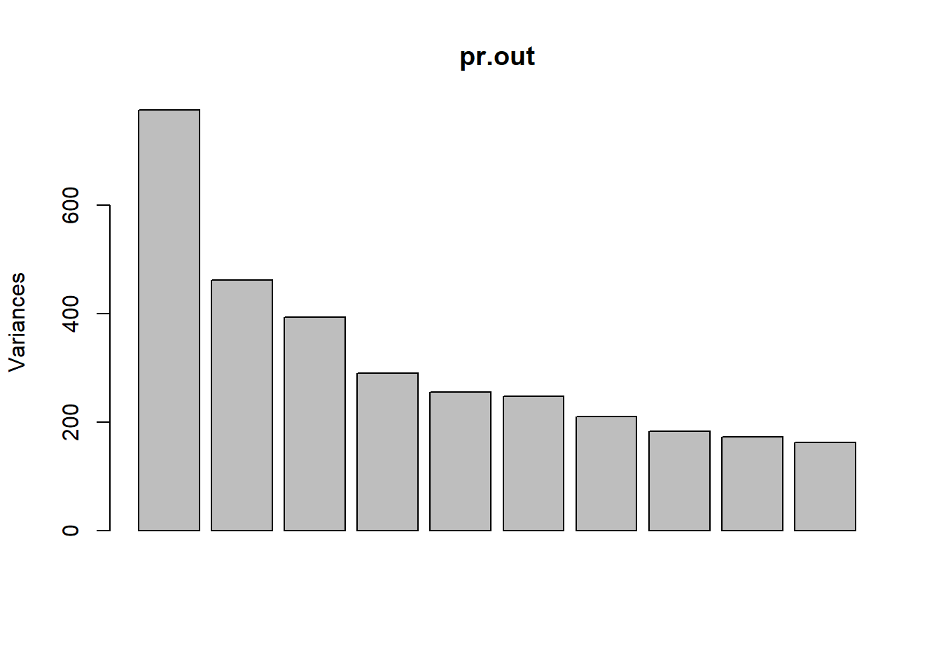
Note that the height of each bar in the bar plot is given by squaring
the corresponding element of pr.out$sdev. However, it is
more informative to plot the PVE of each principal component (i.e. a
scree plot) and the cumulative PVE of each principal component. This can
be done with just a little work.
pve <- 100 * pr.out$sdev^2 / sum(pr.out$sdev^2)
par(mfrow = c(1, 2))
plot(pve,  type = "o", ylab = "PVE",
    xlab = "Principal Component", col = "blue")
plot(cumsum(pve), type = "o", ylab = "Cumulative PVE",
    xlab = "Principal Component", col = "brown3")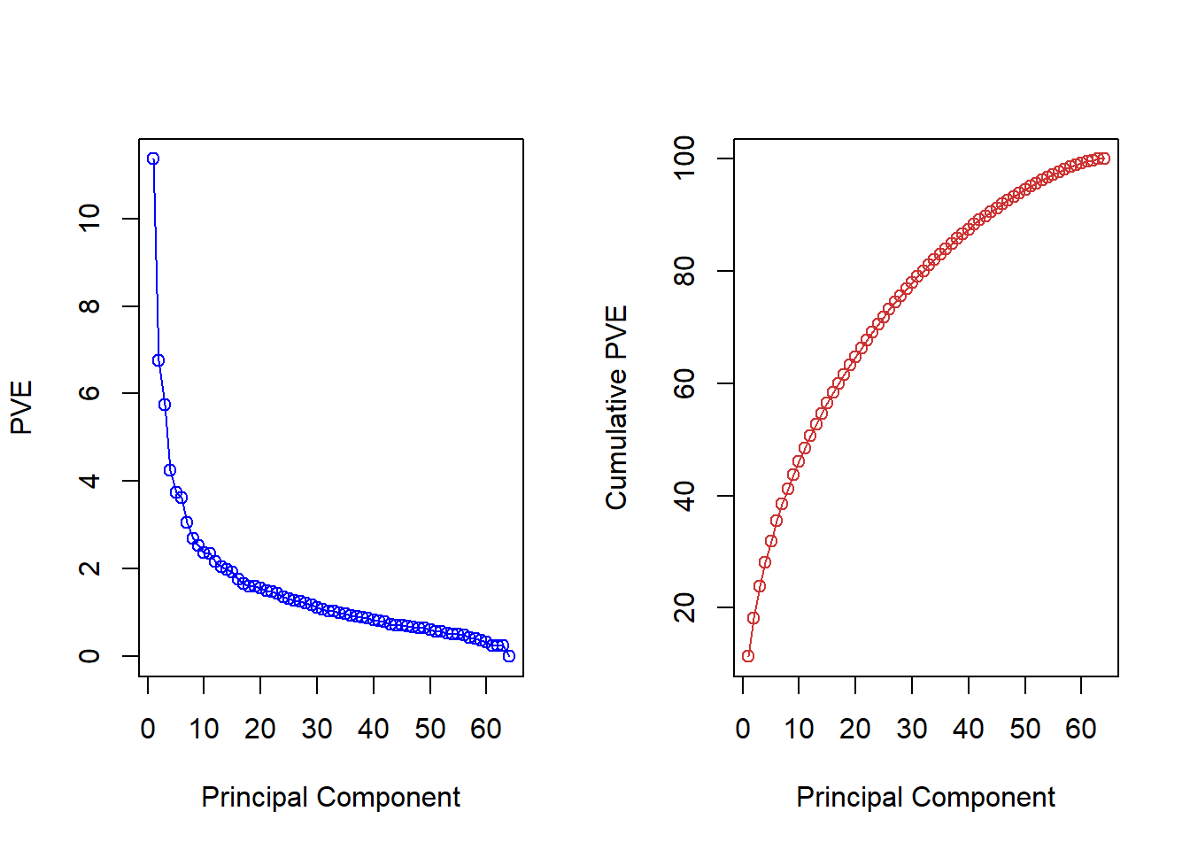
(Note that the elements of pve can also be computed
directly from the summary, summary(pr.out)$importance[2, ],
and the elements of cumsum(pve) are given by
summary(pr.out)$importance[3, ].)
We see that together, the first seven principal components explain around 40% of the variance in the data. This is not a huge amount of the variance. However, looking at the scree plot, we see that while each of the first seven principal components explain a substantial amount of variance, there is a marked decrease in the variance explained by further principal components. That is, there is an elbow in the plot after approximately the seventh principal component. This suggests that there may be little benefit to examining more than seven or so principal components (though even examining seven principal components may be difficult).
Rather than performing hierarchical clustering on the entire data matrix, we can simply perform hierarchical clustering on the first few principal component score vectors, as follows:
hc.out <- hclust(dist(pr.out$x[, 1:5]))
plot(hc.out, labels = nci.labs,
    main = "Hier. Clust. on First Five Score Vectors")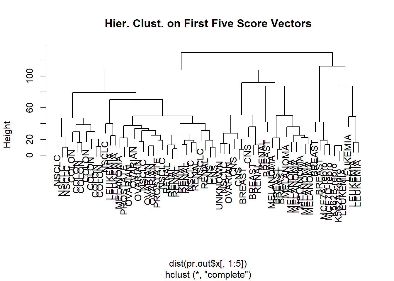
table(cutree(hc.out, 4), nci.labs)## nci.labs
## BREAST CNS COLON K562A-repro K562B-repro LEUKEMIA MCF7A-repro MCF7D-repro
## 1 0 2 7 0 0 2 0 0
## 2 5 3 0 0 0 0 0 0
## 3 0 0 0 1 1 4 0 0
## 4 2 0 0 0 0 0 1 1
## nci.labs
## MELANOMA NSCLC OVARIAN PROSTATE RENAL UNKNOWN
## 1 1 8 5 2 7 0
## 2 7 1 1 0 2 1
## 3 0 0 0 0 0 0
## 4 0 0 0 0 0 0Not surprisingly, these results are different from the ones that we obtained when we performed hierarchical clustering on the full data set:
hc.out <- hclust(dist(scale(nci.data)))
hc.clusters <- cutree(hc.out, 4)
table(hc.clusters, nci.labs)
## nci.labs
## hc.clusters BREAST CNS COLON K562A-repro K562B-repro LEUKEMIA MCF7A-repro
## 1 2 3 2 0 0 0 0
## 2 3 2 0 0 0 0 0
## 3 0 0 0 1 1 6 0
## 4 2 0 5 0 0 0 1
## nci.labs
## hc.clusters MCF7D-repro MELANOMA NSCLC OVARIAN PROSTATE RENAL UNKNOWN
## 1 0 8 8 6 2 8 1
## 2 0 0 1 0 0 1 0
## 3 0 0 0 0 0 0 0
## 4 1 0 0 0 0 0 0Sometimes performing clustering on the first few principal component score vectors can give better results than performing clustering on the full data. In this situation, we might view the principal component step as one of denoising the data. We could also perform \(K\)-means clustering on the first few principal component score vectors rather than the full data set.